Nowadays, with the rapid development of rail transportation systems, passenger demand and the possibility of the risks occurring in this industry have increased. These conditions cause uncertainty in passenger demand and the development of adverse impacts as a result of risks, which put the assurance of precise planning in jeopardy. To deal with uncertainty and lessen negative impacts, robust optimization of the train scheduling problem in the presence of risks is crucial. A two-stage mixed integer programming model is suggested in this study. In the first stage, the objective of the nominal train scheduling problem is to minimize the total travel time function and optimally determine the decision variables of the train timetables and the number of train stops. A robust optimization model is developed in the second stage with the aim of minimizing unsatisfied demand and reducing passenger dissatisfaction. Additionally, programming is carried out and the set of optimal risk response actions is identified in the proposed approach for the presence of primary and secondary risks in the train scheduling problem. A real-world example is provided to demonstrate the model's effectiveness and to compare the developed models. The results demonstrate that secondary risk plays a significant role in the process of optimal response actions selection. Furthermore, in the face of uncertainty, robust solutions can significantly and effectively minimize unsatisfied demand by a slightly rise in the travel time and the number of stops obtained from the nominal problem.
Citation: Shirin Ramezan Ghanbari, Behrouz Afshar-Nadjafi, Majid Sabzehparvar. Robust optimization of train scheduling with consideration of response actions to primary and secondary risks[J]. Mathematical Biosciences and Engineering, 2023, 20(7): 13015-13035. doi: 10.3934/mbe.2023580
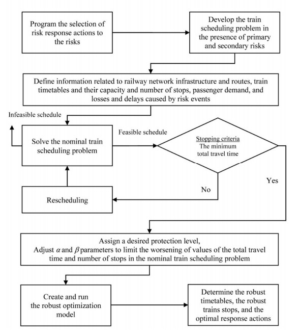
Nowadays, with the rapid development of rail transportation systems, passenger demand and the possibility of the risks occurring in this industry have increased. These conditions cause uncertainty in passenger demand and the development of adverse impacts as a result of risks, which put the assurance of precise planning in jeopardy. To deal with uncertainty and lessen negative impacts, robust optimization of the train scheduling problem in the presence of risks is crucial. A two-stage mixed integer programming model is suggested in this study. In the first stage, the objective of the nominal train scheduling problem is to minimize the total travel time function and optimally determine the decision variables of the train timetables and the number of train stops. A robust optimization model is developed in the second stage with the aim of minimizing unsatisfied demand and reducing passenger dissatisfaction. Additionally, programming is carried out and the set of optimal risk response actions is identified in the proposed approach for the presence of primary and secondary risks in the train scheduling problem. A real-world example is provided to demonstrate the model's effectiveness and to compare the developed models. The results demonstrate that secondary risk plays a significant role in the process of optimal response actions selection. Furthermore, in the face of uncertainty, robust solutions can significantly and effectively minimize unsatisfied demand by a slightly rise in the travel time and the number of stops obtained from the nominal problem.

| [1] |
G. J. Read, A. Naweed, P. M. Salmon, Complexity on the rails: A systems-based approach to understanding safety management in rail transport, Reliab. Eng. Syst. Saf., 188 (2019), 352–365. https://doi.org/10.1016/j.ress.2019.03.038 doi: 10.1016/j.ress.2019.03.038

|
| [2] |
E. Zio, The future of risk assessment, Reliab. Eng. Syst. Saf., 177 (2018), 176–190. https://doi.org/10.1016/j.ress.2018.04.020 doi: 10.1016/j.ress.2018.04.020
|
| [3] |
A. Di Graziano, V. Marchetta, J. Grande, S, Fiore, Application of a decision support tool for the risk management of a metro system, Int. J. Rail Transp., 10 (2022), 352–374. https://doi.org/10.1080/23248378.2021.1906341 doi: 10.1080/23248378.2021.1906341
|
| [4] |
V. Tummala, J. F. Burchett, Applying a risk management process (RMP) to manage cost risk for an EHV transmission line project, Int. J. Project Manage., 17 (1999), 223–235. https://doi.org/10.1016/S0263-7863(98)00038-6 doi: 10.1016/S0263-7863(98)00038-6
|
| [5] | A. Malik, K. Ullah, Risk and its mitigation techniques, in Introduction to Takafu, Springer Nature, (2019), 45–51. https://doi.org/10.1007/978-981-32-9016-7_4 |
| [6] |
Z. Feng, C. Cao, A. Mostafizi, H. Wang, X. Chang, Uncertain demand based integrated optimisation for train timetabling and coupling on the high-speed rail network, Int. J. Prod. Res., 61 (2023), 1532–1555. https://doi.org/10.1080/00207543.2022.2042415 doi: 10.1080/00207543.2022.2042415
|
| [7] |
S. Singh, M. B. Biswal, A robust optimization model under uncertain environment: An application in production planning, Comput. Ind. Eng., 155 (2021), 107169. https://doi.org/10.1016/j.cie.2021.107169 doi: 10.1016/j.cie.2021.107169
|
| [8] |
R. Bubbico, S. Di Cave, B. Mazzarotta, Risk analysis for road and rail transport of hazardous materials: a GIS approach, J. Loss Prev. Process Ind., 17 (2004), 483–488. https://doi.org/10.1016/j.jlp.2004.08.011 doi: 10.1016/j.jlp.2004.08.011
|
| [9] |
M. R. Saat, C. Barkan, Generalized railway tank car safety design optimization for hazardous materials transport: Addressing the trade-off between transportation efficiency and safety, J. Hazard. Mater., 189 (2011), 62–68. https://doi.org/10.1016/j.jhazmat.2011.01.136 doi: 10.1016/j.jhazmat.2011.01.136
|
| [10] |
Q. Tian, H. Wang, Optimization of preventive maintenance schedule of subway train components based on a game model from the perspective of failure risk, Sustainable Cities Soc., 81 (2022), 103819. https://doi.org/10.1016/j.scs.2022.103819 doi: 10.1016/j.scs.2022.103819
|
| [11] |
R. L. Burdett, E. Kozan, Scheduling trains on parallel lines with crossover points, J. Intell. Transp. Syst., 13 (2009), 171–187. https://doi.org/10.1080/15472450903297608 doi: 10.1080/15472450903297608
|
| [12] |
Ö. Yalçınkaya, G. M. Bayhan, A feasible timetable generator simulation modelling framework for train scheduling problem, Simul. Model. Pract. Theory, 20 (2012), 124–141. https://doi.org/10.1016/j.simpat.2011.09.005 doi: 10.1016/j.simpat.2011.09.005
|
| [13] |
X. Li, H. K. Lo, Energy minimization in dynamic train scheduling and control for metro rail operations, Transp. Res. Part B Methodol., 70 (2014), 269–284. https://doi.org/10.1016/j.trb.2014.09.009 doi: 10.1016/j.trb.2014.09.009
|
| [14] |
Y. Wang, Z. Liao, T. Tang, B. Ning, Train scheduling and circulation planning in urban rail transit lines, Control Eng. Pract., 61 (2017), 112–123. https://doi.org/10.1016/j.conengprac.2017.02.006 doi: 10.1016/j.conengprac.2017.02.006
|
| [15] |
P. Mo, L. Yang, Y. Wang, J. Qi, A flexible metro train scheduling approach to minimize energy cost and passenger waiting time, Comput. Ind. Eng., 132 (2019), 412–432. https://doi.org/10.1016/j.cie.2019.04.031 doi: 10.1016/j.cie.2019.04.031
|
| [16] |
P. Rokhforoz, O. Fink, Hierarchical multi-agent predictive maintenance scheduling for trains using price-based approach, Comput. Ind. Eng., 159 (2021), 107475. https://doi.org/10.1016/j.cie.2021.107475 doi: 10.1016/j.cie.2021.107475
|
| [17] | M. Komeili, P. Nazarian, A. Safari, M. Moradlou, Robust optimal scheduling of CHP-based microgrids in presence of wind and photovoltaic generation units: An IGDT approach, Sustainable Cities Soc., 78 (2022), 103566. https://doi.org/10.1016/j.scs.2021.103566 |
| [18] |
L. Kroon, G. Maróti, M. R. Helmrich, M. Vromans, R. Dekker, Stochastic improvement of cyclic railway timetables, Transp. Res. Part B Methodol., 42 (2008), 553–570. https://doi.org/10.1016/j.trb.2007.11.002 doi: 10.1016/j.trb.2007.11.002
|
| [19] |
S. Li, L. Yang, K. Li, Z. Gao, Robust sampled-data cruise control scheduling of high-speed train, Transp. Res. Part C Emerging Technol., 46 (2014), 274–283. https://doi.org/10.1016/j.trc.2014.06.004 doi: 10.1016/j.trc.2014.06.004
|
| [20] |
A. Jamili, M. P. Aghaee, Robust stop-skipping patterns in urban railway operations under traffic alteration situation, Transp. Res. Part C Emerging Technol, 61 (2015), 63–74. https://doi.org/10.1016/j.trc.2015.09.013 doi: 10.1016/j.trc.2015.09.013
|
| [21] |
P. Jovanović, P. Kecman, N. Bojović, D. Mandić, Optimal allocation of buffer times to increase train schedule robustness, Eur. J. Oper. Res., 256 (2017), 44–54. https://doi.org/10.1016/j.ejor.2016.05.013 doi: 10.1016/j.ejor.2016.05.013
|
| [22] |
F. Rajabighamchi, E. M. Hosein Hajlou, E. Hassannayebi, A multi-objective optimization model for robust skip-stop scheduling with earliness and tardiness penalties, Urban Rail Transit, 5 (2019), 172–185. https://doi.org/10.1007/s40864-019-00108-0 doi: 10.1007/s40864-019-00108-0
|
| [23] |
L. Zhou, X. Yang, H. Wang, J. Wu, L. Chen, H. Yin, et al., A robust train timetable optimization approach for reducing the number of waiting passengers in metro systems, Phys. A Stat. Mech. Appl., 558 (2020), 124927. https://doi.org/10.1016/j.physa.2020.124927 doi: 10.1016/j.physa.2020.124927
|
| [24] |
V. Cacchiani, J. Qi, L. Yang, Robust optimization models for integrated train stop planning and timetabling with passenger demand uncertainty, Transp. Res. Part B Methodol., 136 (2020), 1–29. https://doi.org/10.1016/j.trb.2020.03.009 doi: 10.1016/j.trb.2020.03.009
|
| [25] |
J. Qi, S. Li, Y. Gao, K. Yang, P. Liu, Joint optimization model for train scheduling and train stop planning with passengers' distribution on railway corridors, J. Oper. Res. Soc., 69 (2018), 556–570. https://doi.org/10.1057/s41274-017-0248-x doi: 10.1057/s41274-017-0248-x
|
| [26] | M. Fischetti, M. Monaci, Light robustness, in Robust and online large-scale optimization, Springer, (2009), 61–84. |


Figures(3) / Tables(10)

Shirin Ramezan Ghanbari, Behrouz Afshar-Nadjafi, Majid Sabzehparvar. Robust optimization of train scheduling with consideration of response actions to primary and secondary risks[J]. Mathematical Biosciences and Engineering, 2023, 20(7): 13015-13035. doi: 10.3934/mbe.2023580


 DownLoad: