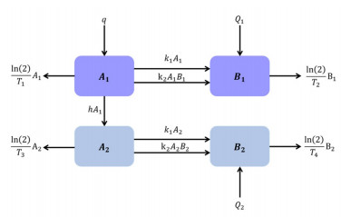
This study aims to analyze a mathematical model of alpha-synuclein transport and aggregation in neurons qualitatively. Our analysis yielded a unique equilibrium point, which exists always. Also, we derive the criteria for the local and global asymptotic stability of the equilibrium. Moreover, we utilize the closed form of the equilibrium to investigate the effect of the models' parameters on decreasing the long term value of the misfolded alpha-synuclein, which may help in suggesting pharmacological interventions for Parkinson's disease. Furthermore, numerical simulations are illustrated to support the analytic results and sensitivity analysis.
Citation: Salma Al-Tuwairqi, Asma Badrah. A qualitative analysis of a model on alpha-synuclein transport and aggregation in neurons[J]. Mathematical Modelling and Control, 2023, 3(2): 104-115. doi: 10.3934/mmc.2023010
This study aims to analyze a mathematical model of alpha-synuclein transport and aggregation in neurons qualitatively. Our analysis yielded a unique equilibrium point, which exists always. Also, we derive the criteria for the local and global asymptotic stability of the equilibrium. Moreover, we utilize the closed form of the equilibrium to investigate the effect of the models' parameters on decreasing the long term value of the misfolded alpha-synuclein, which may help in suggesting pharmacological interventions for Parkinson's disease. Furthermore, numerical simulations are illustrated to support the analytic results and sensitivity analysis.

| [1] |
S. G. Reich, J. M. Savitt, Parkinson's Disease, Med. Clin. N. Am., 103 (2019), 337–350. https://doi.org/10.1016/j.mcna.2018.10.014 doi: 10.1016/j.mcna.2018.10.014

|
| [2] |
M. J. Benskey, R. G. Perez, F. P. Manfredsson, The contribution of alpha synuclein to neuronal survival and function-Implications for Parkinson's disease, J. Neurochem., 137 (2016), 331–359. https://doi.org/10.1111/jnc.13570 doi: 10.1111/jnc.13570
|
| [3] |
S. Mehra, S. Sahay, S. K. Maji, $\alpha$-Synuclein misfolding and aggregation: Implications in Parkinson's disease pathogenesis, BBA-PROTEINS PROTEOM., 1867 (2019), 890–908. https://doi.org/10.1016/j.bbapap.2019.03.001 doi: 10.1016/j.bbapap.2019.03.001
|
| [4] |
R. M. Meade, D. P. Fairlie, J. M. Mason, Alpha-synuclein structure and Parkinson's disease, Mol. Neurodegener., 14 (2019), 3. https://doi.org/10.1186/s13024-018-0304-2 doi: 10.1186/s13024-018-0304-2
|
| [5] |
A. Lloret-Villas, T. M. Varusai, N. Juty, C. Laibe, N. Le Novere, H. Hermjakob, et al., The impact of mathematical modeling in understanding the mechanisms underlying neurodegeneration: Evolving dimensions and future directions, CPT: Pharmacometrics and Systems Pharmacology, 6 (2017), 73–86. https://doi.org/10.1002/psp4.12155 doi: 10.1002/psp4.12155
|
| [6] |
Y. Sarbaz, H. Pourakbari, A review of presented mathematical models in Parkinson's disease: black- and gray-box models, Med. Biol. Eng. Comput., 54 (2016), 855–868. https://doi.org/10.1007/s11517-015-1401-9 doi: 10.1007/s11517-015-1401-9
|
| [7] |
S. Bakshi, V. Chelliah, C. Chen, P. H. van der Graaf, Mathematical Biology Models of Parkinson's Disease, CPT: Pharmacometrics and Systems Pharmacology, 8 (2019), 77–86. https://doi.org/10.1002/psp4.12362 doi: 10.1002/psp4.12362
|
| [8] |
F. Francis, M. R. García, R. H. Middleton, A single compartment model of pacemaking in dissasociated Substantia nigra neurons: Stability and energy analysis, J. Comput. Neurosci., 35 (2013), 295–316. https://doi.org/10.1007/s10827-013-0453-9 doi: 10.1007/s10827-013-0453-9
|
| [9] |
I. A. Kuznetsov, A. V. Kuznetsov, What can trigger the onset of Parkinson's disease - A modeling study based on a compartmental model of $\alpha$-synuclein transport and aggregation in neurons, Math. Biosci., 278 (2016), 22–29. https://doi.org/10.1016/j.mbs.2016.05.002 doi: 10.1016/j.mbs.2016.05.002
|
| [10] |
I. A. Kuznetsov, A. V. Kuznetsov, Mathematical models of $\alpha$-synuclein transport in axons, Comput. Methods Biomech. Biomed. Eng., 19 (2016), 515–526. https://doi.org/10.1080/10255842.2015.1043628 doi: 10.1080/10255842.2015.1043628
|
| [11] |
K. Sneppen, L. Lizana, M. H. Jensen, S. Pigolotti, D. Otzen, Modeling proteasome dynamics in Parkinson's disease, Phys. Biol., 6 (2009), 036005. https://doi.org/10.1088/1478-3975/6/3/036005 doi: 10.1088/1478-3975/6/3/036005
|
| [12] | M. W. Hirsch, S. Smale, R. L. Devaney, Differential Equations, Dynamical Systems, and an Introduction to Chaos, Boston: Academic Press, third edition, 2013. |
| [13] | L. Perko, Differential equations and dynamical systems, vol. 7. Springer Science & Business Media, 2013. |
| [14] | M. Martcheva, An introduction to mathematical epidemiology, Springer, 2015. |
| [15] | M. Nagumo, Über die lage der integralkurven gewöhnlicher differentialgleichungen, Proceedings of the Physico-Mathematical Society of Japan. 3rd Series, 24 (1942), 551–559. |
| [16] | J.-M. Bony, Principe du maximum, inégalité de harnack et unicité du probleme de cauchy pour les opérateurs elliptiques dégénérés, Annales de l'institut Fourier, 19 (1969), 277–304. |
| [17] | H. Brezis, On a characterization of flow-invariant sets, Comm. Pure Appl. Math., 223 (1970), 261–263. |
| [18] |
J. Li, Y. Xiao, F. Zhang, Y. Yang, An algebraic approach to proving the global stability of a class of epidemic models, Nonlinear Anal.-Real, 13 (2012), 2006–2016. https://doi.org/10.1016/j.nonrwa.2011.12.022 doi: 10.1016/j.nonrwa.2011.12.022
|


Figures(4) / Tables(3)
Salma Al-Tuwairqi, Asma Badrah. A qualitative analysis of a model on alpha-synuclein transport and aggregation in neurons[J]. Mathematical Modelling and Control, 2023, 3(2): 104-115. doi: 10.3934/mmc.2023010


 DownLoad: