Compared to many infectious diseases, tuberculosis has a high mortality rate. Because of this, a great deal of illustrative research has been done on the modeling and study of tuberculosis using mathematics. In this work, a mathematical model is created by taking into account the underlying presumptions of this disease. One of the main novelties of the paper is to consider two different treatment strategies namely protective treatment for the latent populations from the disease and the main treatment applied to the infected populations. This situation can be regarded as the other novelty of the paper. The susceptible, latent, infected, and recovered populations, as well as the two mentioned treatment classes, are all included in the proposed six-dimensional model's compartmental framework. Additionally, a region that is biologically possible is presented, as well as the solution's positivity, existence, and uniqueness. The suggested model's solutions are carried out as numerical simulations using assumed and literature-based parameter values and analyzing its graphics. To get the results, a fourth-order Runge-Kutta numerical approach is used.
Citation: Mehmet Yavuz, Fatma Özköse, Müzeyyen Akman, Zehra Tuğba Taştan. A new mathematical model for tuberculosis epidemic under the consciousness effect[J]. Mathematical Modelling and Control, 2023, 3(2): 88-103. doi: 10.3934/mmc.2023009
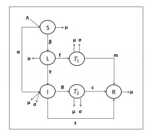
Compared to many infectious diseases, tuberculosis has a high mortality rate. Because of this, a great deal of illustrative research has been done on the modeling and study of tuberculosis using mathematics. In this work, a mathematical model is created by taking into account the underlying presumptions of this disease. One of the main novelties of the paper is to consider two different treatment strategies namely protective treatment for the latent populations from the disease and the main treatment applied to the infected populations. This situation can be regarded as the other novelty of the paper. The susceptible, latent, infected, and recovered populations, as well as the two mentioned treatment classes, are all included in the proposed six-dimensional model's compartmental framework. Additionally, a region that is biologically possible is presented, as well as the solution's positivity, existence, and uniqueness. The suggested model's solutions are carried out as numerical simulations using assumed and literature-based parameter values and analyzing its graphics. To get the results, a fourth-order Runge-Kutta numerical approach is used.

| [1] | World Health Organization Weakly Report, 2021. Available from: https://www.who.int/publications/i/item/9789240013131. |
| [2] |
D. Young, J. Stark, D. Kirschner, Systems Biology of Persistent Infection: Tuberculosis as a Case Study, Nat. Rev. Microbiol., 6 (2008), 520–528. https://doi.org/10.1038/nrmicro1919 doi: 10.1038/nrmicro1919

|
| [3] | Ministry of Health, 2021. Available from: https://hsgm.saglik.gov.tr/tr/tuberkuloz-haberler/24-mart-dunya-tuberkuloz-gunu-etkinlikleri.html. |
| [4] |
H. Waaler, A. Geser, S. Andersen, The Use of Mathematical Models in the Study of the Epidemiology of Tuberculosis, American Journal of Public Health and the Nations Health, 52 (1962), 1002–1013. https://doi.org/10.2105/ajph.52.6.1002 doi: 10.2105/ajph.52.6.1002
|
| [5] |
M. Schulzer, M. P. Radhamani, S. Grzybowski, E. Mak, J. M. Fitzgerald, A Mathematical Model for the Prediction of the İmpact of HIV İnfection on Tuberculosis, Int. J. Epidemiol., 23 (1994), 400–407. https://doi.org/10.1093/ije/23.2.400 doi: 10.1093/ije/23.2.400
|
| [6] |
C. Castillo-Chavez, Z. Feng, To Treat or Not to Treat: The Case of Tuberculosis, J. Math. Biol., 35 (1997), 629–656. https://doi.org/10.1007/s002850050069 doi: 10.1007/s002850050069
|
| [7] |
Z. Feng, C. Castillo-Chavez, A. F. Capurro, A Model for Tuberculosis with Exogenous Reinfection, Theor. Popul. Biol., 57 (2000), 235–247. https://doi.org/10.1006/tpbi.2000.1451 doi: 10.1006/tpbi.2000.1451
|
| [8] |
T. Gumbo, A. Louie, M. R. Deziel, L. M. Parsons, M. Salfinger, G. L. Drusano, Selection of a Moxifloxacin Dose That Suppresses Drug Resistance in Mycobacterium Tuberculosis, by Use of an in Vitro Pharmacodynamic Infection Model and Mathematical Modeling, J. Infect. Dis., 190 (2004), 1642–1651. https://doi.org/10.1086/424849 doi: 10.1086/424849
|
| [9] |
D. W. Dowdy, R. E. Chaisson, L. H. Moulton, S. E. Dorman, The Potential Impact of Enhanced Diagnostic Techniques for Tuberculosis Driven by Hiv: A Mathematical Model, Aids, 20 (2006), 751–762. https://doi.org/10.1097/01.aids.0000216376.07185.cc doi: 10.1097/01.aids.0000216376.07185.cc
|
| [10] |
D. W. Dowdy, R. E. Chaisson, G. Maartens, E. L. Corbett, S. E. Dorman, Impact of enhanced tuberculosis diagnosis in South Africa: a mathematical model of expanded culture and drug susceptibility testing, Proceedings of the National Academy of Sciences, 105 (2008), 11293–11298. https://doi.org/10.1073/pnas.0800965105 doi: 10.1073/pnas.0800965105
|
| [11] |
S. Bowong, J. J. Tewa, Mathematical Analysis of a Tuberculosis Model with Differential Infectivity, Commun. Nonlinear Sci., 14 (2009), 4010–4021. https://doi.org/10.1016/j.cnsns.2009.02.017 doi: 10.1016/j.cnsns.2009.02.017
|
| [12] |
J. Liu, T. Zhang, Global Stability for a Tuberculosis Model, Math. Comput. Model., 54 (2011), 836–845. https://doi.org/10.1016/j.mcm.2011.03.033 doi: 10.1016/j.mcm.2011.03.033
|
| [13] |
J. J. Tewa, S. Bowong, S. O. Noutchie, Mathematical Analysis of a Two-Patch Model of Tuberculosis Disease with Staged Progression, Appl. Math. Model., 36 (2012), 5792–5807. https://doi.org/10.1016/j.apm.2012.01.026 doi: 10.1016/j.apm.2012.01.026
|
| [14] |
J. M. Trauer, J. T. Denholm, E. S. McBryde, Construction of a Mathematical Model for Tuberculosis Transmission in Highly Endemic Regions of the Asia-Pacific, J. Theor. Biol., 358 (2014), 74–84. https://doi.org/10.1016/j.jtbi.2014.05.023 doi: 10.1016/j.jtbi.2014.05.023
|
| [15] |
B. K. Mishra, J. Srivastava, Mathematical Model on Pulmonary and Multidrug-Resistant Tuberculosis Patients with Vaccination, Journal of the Egyptian Mathematical Society, 22 (2014), 311–316. https://doi.org/10.1016/j.joems.2013.07.006 doi: 10.1016/j.joems.2013.07.006
|
| [16] |
J. Li, Y. Zhang, X. Zhang, Mathematical Modeling of Tuberculosis Data of China, J. Theor. Biol., 365 (2015), 159–163. https://doi.org/10.1016/j.jtbi.2014.10.019 doi: 10.1016/j.jtbi.2014.10.019
|
| [17] |
P. J. Dodd, C. Sismanidis, J. A. Seddon, Global Burden of Drug-Resistant Tuberculosis in Children: A Mathematical Modelling Study, The Lancet infectious diseases, 16 (2016), 1193–1201. https://doi.org/10.1016/S1473-3099(16)30132-3 doi: 10.1016/S1473-3099(16)30132-3
|
| [18] | A. A. B. Sy, M. L. Diagne, I. Mbaye, O. Seydic, A Mathematical Model for the Impact of Public Health Education Campaign for Tuberculosis, Far East Journal of Applied Mathematics, 100 (2018), 97–138. https://doi.org/10.17654AM100020097 |
| [19] |
D. N. Vinh, D. T. M. Ha, N. T. Hanh, G. Thwaites, M. F. Boni, H. E. Clapham, et al., Modeling Tuberculosis Dynamics with the Presence of Hyper-Susceptible Individuals for Ho Chi Minh City from 1996 to 2015, BMC Infect. Dis., 18 (2018), 494. https://doi.org/10.1186/s12879-018-3383-3 doi: 10.1186/s12879-018-3383-3
|
| [20] |
K. C. Chong, C. C. Leung, W. W. Yew, B. C. Y. Zee, G. C. H. Tam, M. H. Wang, et al., Mathematical modelling of the impact of treating latent tuberculosis infection in the elderly in a city with intermediate tuberculosis burden, Scientific reports, 9 (2019), 1–11. https://doi.org/10.1038/s41598-019-41256-4 doi: 10.1038/s41598-019-41256-4
|
| [21] |
P. A. Naik, M. Yavuz, S. Zu, J. Qureshi, S. Townley, Modeling and analysis of COVID-19 epidemics with treatment in fractional derivatives using real data from Pakistan, The European Physical Journal Plus, 135 (2020), 1–42. https://doi.org/10.1140/epjp/s13360-020-00819-5 doi: 10.1140/epjp/s13360-020-00819-5
|
| [22] |
S. Allegretti, I. M. Bulai, R. Marino, M. A. Menandro, K. Parisi, Vaccination effect conjoint to fraction of avoided contacts for a Sars-Cov-2 mathematical model, Mathematical Modelling and Numerical Simulation with Applications, 1 (2021), 56–66. https://doi.org/10.53391/mmnsa.2021.01.006 doi: 10.53391/mmnsa.2021.01.006
|
| [23] |
F. Özköse, M. Yavuz, Investigation of interactions between COVID-19 and diabetes with hereditary traits using real data: A case study in Turkey, Comput. Biol. Med., 141 (2022), 105044. https://doi.org/10.1016/j.compbiomed.2021.105044 doi: 10.1016/j.compbiomed.2021.105044
|
| [24] |
R. Ikram, A. Khan, M. Zahri, A. Saeed, M. Yavuz, P. Kumam, Extinction and stationary distribution of a stochastic COVID-19 epidemic model with time-delay, Comput. Biol. Med., 141 (2022), 105115. https://doi.org/10.1016/j.compbiomed.2021.105115 doi: 10.1016/j.compbiomed.2021.105115
|
| [25] |
Y. Sabbar, D. Kiouach, S. P. Rajasekar, S. E. A. El-Idrissi, The influence of quadratic Lévy noise on the dynamic of an SIC contagious illness model: New framework, critical comparison and an application to COVID-19 (SARS-CoV-2) case, Chaos, Solitons & Fractals, 159 (2022), 112110. https://doi.org/10.1016/j.chaos.2022.112110 doi: 10.1016/j.chaos.2022.112110
|
| [26] |
M. Higazy, Novel fractional order SIDARTHE mathematical model of COVID-19 pandemic, Chaos, Solitons & Fractals, 138 (2020), 110007. https://doi.org/10.1016/j.chaos.2020.110007 doi: 10.1016/j.chaos.2020.110007
|
| [27] |
Z. H. Shen, Y. M. Chu, M. A. Khan, S. Muhammad, O. A. Al-Hartomy, M. Higazy, Mathematical modeling and optimal control of the COVID-19 dynamics, Results Phys., 31 (2021), 105028. https://doi.org/10.1016/j.rinp.2021.105028 doi: 10.1016/j.rinp.2021.105028
|
| [28] |
M. Higazy, M. A. Alyami, New Caputo-Fabrizio fractional order SEIASqEqHR model for COVID-19 epidemic transmission with genetic algorithm based control strategy, Alex. Eng. J., 59 (2020), 4719–4736. https://doi.org/10.1016/j.aej.2020.08.034 doi: 10.1016/j.aej.2020.08.034
|
| [29] |
M. Higazy, F. M. Allehiany, E. E. Mahmoud, Numerical study of fractional order COVID-19 pandemic transmission model in context of ABO blood group, Results Phys., 22 (2021), 103852. https://doi.org/10.1016/j.rinp.2021.103852 doi: 10.1016/j.rinp.2021.103852
|
| [30] |
S. Ahmad, D. Qiu, M. ur Rahman, Dynamics of a fractional-order COVID-19 model under the nonsingular kernel of Caputo-Fabrizio operator, Mathematical Modelling and Numerical Simulation with Applications, 2 (2022), 228–243. https://doi.org/10.53391/mmnsa.2022.019 doi: 10.53391/mmnsa.2022.019
|
| [31] |
A. G. C. Pérez, D. A. Oluyori, A model for COVID-19 and bacterial pneumonia coinfection with community-and hospital-acquired infections, Mathematical Modelling and Numerical Simulation with Applications, 2 (2022), 197–210. https://doi.org/10.53391/mmnsa.2022.016 doi: 10.53391/mmnsa.2022.016
|
| [32] |
A. O. Atede, A. Omame, A., S. C. Inyama, A fractional order vaccination model for COVID-19 incorporating environmental transmission: a case study using Nigerian data. Bulletin of Biomathematics, 1 (2023), 78–110. https://doi.org/10.59292/bulletinbiomath.2023005 doi: 10.59292/bulletinbiomath.2023005
|
| [33] |
F. Özköse, M. T. Şenel, R. Habbireeh, Fractional-order mathematical modelling of cancer cells-cancer stem cells-immune system interaction with chemotherapy, Mathematical Modelling and Numerical Simulation with Applications, 1 (2021), 67–83. https://doi.org/10.53391/mmnsa.2021.01.007 doi: 10.53391/mmnsa.2021.01.007
|
| [34] |
A. M. S. Mahdy, M. Higazy, K. A. Gepreel, A. A. A. El-Dahdouh, Optimal control and bifurcation diagram for a model nonlinear fractional SIRC, Alex. Eng. J., 59 (2020), 3481–3501. https://doi.org/10.1016/j.aej.2020.05.028 doi: 10.1016/j.aej.2020.05.028
|
| [35] |
F. Evirgen, S. Uçar, N. Özdemir, Z. Hammouch, System response of an alcoholism model under the effect of immigration via non-singular kernel derivative, Discrete Cont. Dyn.-S, 14 (2021), 2199. https://doi.org/10.3934/dcdss.2020145 doi: 10.3934/dcdss.2020145
|
| [36] |
P. Kumar, V. S. Erturk, Dynamics of cholera disease by using two recent fractional numerical methods, Mathematical Modelling and Numerical Simulation with Applications, 1 (2021), 102–111. https://doi.org/10.53391/mmnsa.2021.01.010 doi: 10.53391/mmnsa.2021.01.010
|
| [37] |
F. Özköse, R. Habbireeh, M. T. Şenel, A novel fractional order model of SARS-CoV-2 and Cholera disease with real data, J. Comput. Appl. Math., 423 (2023), 114969. https://doi.org/10.1016/j.cam.2022.114969 doi: 10.1016/j.cam.2022.114969
|
| [38] |
H. Joshi, B. K. Jha, Chaos of calcium diffusion in Parkinson's infectious disease model and treatment mechanism via Hilfer fractional derivative, Mathematical Modelling and Numerical Simulation with Applications, 1 (2021), 84–94. https://doi.org/10.53391/mmnsa.2021.01.008 doi: 10.53391/mmnsa.2021.01.008
|
| [39] |
H. Joshi, M. Yavuz, I. Stamova, A fractional order vaccination model for COVID-19 incorporating environmental transmission: a case study using Nigerian data. Bulletin of Biomathematics, 1 (2023), 24–39. https://doi.org/10.59292/bulletinbiomath.2023002 doi: 10.59292/bulletinbiomath.2023002
|
| [40] |
P. A. Naik, K. M. Owolabi, M. Yavuz, J. Zu, Chaotic dynamics of a fractional order HIV-1 model involving AIDS-related cancer cells, Chaos, Solitons & Fractals, 140 (2020), 110272. https://doi.org/10.1016/j.chaos.2020.110272 doi: 10.1016/j.chaos.2020.110272
|
| [41] |
P. A. Naik, M. Yavuz, J. Zu, The role of prostitution on HIV transmission with memory: a modeling approach, Alex. Eng. J., 59 (2020), 2513–2531. https://doi.org/10.1016/j.aej.2020.04.016 doi: 10.1016/j.aej.2020.04.016
|
| [42] |
R. M. Jena, S. Chakraverty, M. Yavuz, T. Abdeljawad, A New Modeling and Existence-Uniqueness Analysis for Babesiosis Disease of Fractional Order, Mod. Phys. Lett. B, (2021). https://doi.org/10.1142/S0217984921504431 doi: 10.1142/S0217984921504431
|
| [43] |
M. Yavuz, N. Sene, Stability Analysis and Numerical Computation of the Fractional Predator–Prey Model with the Harvesting Rate, Fractal Fract., 4 (2020), 35. https://doi.org/10.3390/fractalfract4030035 doi: 10.3390/fractalfract4030035
|
| [44] |
P. A. Naik, Z. Eskandari, M. Yavuz, J. Zu, Complex dynamics of a discrete-time Bazykin–Berezovskaya prey-predator model with a strong Allee effect, J. Comput. Appl. Math., 413 (2022), 114401. https://doi.org/10.1016/j.cam.2022.114401 doi: 10.1016/j.cam.2022.114401
|
| [45] |
M. Naim, Y. Sabbar, A. Zeb, Stability characterization of a fractional-order viral system with the non-cytolytic immune assumption, Mathematical Modelling and Numerical Simulation with Applications, 2 (2022), 164–176. https://doi.org/10.53391/mmnsa.2022.013 doi: 10.53391/mmnsa.2022.013
|
| [46] |
F. Evirgen, Transmission of Nipah virus dynamics under Caputo fractional derivative, J. Comput. Appl. Math., 418 (2023), 114654. https://doi.org/10.1016/j.cam.2022.114654 doi: 10.1016/j.cam.2022.114654
|
| [47] |
Y. Sabbar, A. Khan, A. Din, D. Kiouach, S. P. Rajasekar, Determining the global threshold of an epidemic model with general interference function and high-order perturbation, AIMS Math., 7 (2022), 19865–19890. https://doi.org/10.3934/math.20221088 doi: 10.3934/math.20221088
|
| [48] |
Y. Sabbar, A. Din, D. Kiouach, Predicting potential scenarios for wastewater treatment under unstable physical and chemical laboratory conditions: A mathematical study, Results Phys., 39 (2022), 105717. https://doi.org/10.1016/j.rinp.2022.105717 doi: 10.1016/j.rinp.2022.105717
|
| [49] |
A. R. Sheergojri, P. Iqbal, P. Agarwal, N. Ozdemir, Uncertainty-based Gompertz growth model for tumor population and its numerical analysis, An International Journal of Optimization and Control: Theories & Applications (IJOCTA), 12 (2022), 137–150. https://doi.org/10.11121/ijocta.2022.1208 doi: 10.11121/ijocta.2022.1208
|
| [50] |
Y. Sabbar, M. Yavuz, F. Özköse, Infection Eradication Criterion in a General Epidemic Model with Logistic Growth, Quarantine Strategy, Media Intrusion, and Quadratic Perturbation, Mathematics, 10 (2022), 4213. https://doi.org/10.3390/math10224213 doi: 10.3390/math10224213
|
| [51] |
Z. Hammouch, M. Yavuz, N. Özdemir, Numerical solutions and synchronization of a variable-order fractional chaotic system, Mathematical Modelling and Numerical Simulation with Applications, 1 (2021), 11–23. https://doi.org/10.53391/mmnsa.2021.01.002 doi: 10.53391/mmnsa.2021.01.002
|
| [52] |
Y. Sabbar, A. Zeb, D. Kiouach, N. Gul, T. Sitthiwirattham, D. Baleanu, et al., Dynamical bifurcation of a sewage treatment model with general higher-order perturbation, Results Phys., 39 (2022), 105799. https://doi.org/10.1016/j.rinp.2022.105799 doi: 10.1016/j.rinp.2022.105799
|
| [53] |
S. Kim, A. A. de los Reyes V, E. Jung, Country-specific intervention strategies for top three TB burden countries using mathematical model, PloS one, 15 (2020), e0230964. https://doi.org/10.1371/journal.pone.0230964 doi: 10.1371/journal.pone.0230964
|
| [54] |
S. Ullah, M. A. Khan, M. Farooq, T. Gul, Modeling and analysis of tuberculosis (tb) in Khyber Pakhtunkhwa, Pakistan, Math. Comput. Simulat., 165 (2019), 181–199. https://doi.org/10.1016/j.matcom.2019.03.012 doi: 10.1016/j.matcom.2019.03.012
|
| [55] | C. Obasi, G. C. E. Mbah, On the stability analysis of a mathematical model of Lassa fever disease dynamics, Journal of the Nigerian Society for Mathematical Biology, 2 (2019), 135–144. |
| [56] | G. Birkhoff, G. C. Rota, Ordinary Differential Equations, Wiley: Hoboken, NJ, USA, 1989. |
| [57] |
H. W. Hethcote, The mathematics of infectious diseases, SIAM Rev., 42 (2000), 599–653. https://doi.org/10.1137/S0036144500371907 doi: 10.1137/S0036144500371907
|
| [58] |
P. Van den Driessche, J. Watmough, Reproduction numbers and sub-threshold endemic equilibria for compartmental models of disease transmission, Math. Biosci., 180 (2002), 29–48. https://doi.org/10.1016/S0025-5564(02)00108-6 doi: 10.1016/S0025-5564(02)00108-6
|
| [59] |
E. Ahmed, A. S. Elgazzar, On fractional order differential equations model for nonlocal epidemics, Physica A, 379 (2007), 607–614. https://doi.org/10.1016/j.physa.2007.01.010 doi: 10.1016/j.physa.2007.01.010
|
| [60] | F. Brauer, C. Castillo-Chavez, Z. Feng, Mathematical models in epidemiology, Vol. 32, 2019, New York: Springer. |


Figures(6) / Tables(1)
Mehmet Yavuz, Fatma Özköse, Müzeyyen Akman, Zehra Tuğba Taştan. A new mathematical model for tuberculosis epidemic under the consciousness effect[J]. Mathematical Modelling and Control, 2023, 3(2): 88-103. doi: 10.3934/mmc.2023009


 DownLoad: