We consider a low Reynolds number artificial swimmer that consists of an active arm followed by $ N $ passive springs separated by spheres. This setup generalizes an approach proposed in Montino and DeSimone, Eur. Phys. J. E, vol. 38, 2015. We further study the limit as the number of springs tends to infinity and the parameters are scaled conveniently, and provide a rigorous proof of the convergence of the discrete model to the continuous one. Several numerical experiments show the performances of the displacement in terms of the frequency or the amplitude of the oscillation of the active arm.
Citation: François Alouges, Aline Lefebvre-Lepot, Jessie Levillain. A limiting model for a low Reynolds number swimmer with $ N $ passive elastic arms[J]. Mathematics in Engineering, 2023, 5(5): 1-20. doi: 10.3934/mine.2023087
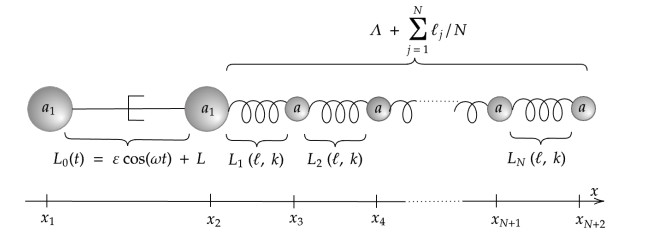
We consider a low Reynolds number artificial swimmer that consists of an active arm followed by $ N $ passive springs separated by spheres. This setup generalizes an approach proposed in Montino and DeSimone, Eur. Phys. J. E, vol. 38, 2015. We further study the limit as the number of springs tends to infinity and the parameters are scaled conveniently, and provide a rigorous proof of the convergence of the discrete model to the continuous one. Several numerical experiments show the performances of the displacement in terms of the frequency or the amplitude of the oscillation of the active arm.

| [1] |
F. Alouges, A. DeSimone, A. Lefebvre, Optimal strokes for low Reynolds number swimmers: an example, J. Nonlinear Sci., 18 (2008), 277–302. https://doi.org/10.1007/s00332-007-9013-7 doi: 10.1007/s00332-007-9013-7

|
| [2] |
F. Alouges, A. DeSimone, A. Lefebvre, Optimal strokes for axisymmetric microswimmers, Eur. Phys. J. E, 28 (2009), 279–284. https://doi.org/10.1140/epje/i2008-10406-4 doi: 10.1140/epje/i2008-10406-4
|
| [3] |
F. Alouges, A. DeSimone, L. Heltai, Numerical strategies for stroke optimization of axisymmetric microswimmers, Math. Mod. Meth. Appl. Sci., 21 (2011), 361–387. https://doi.org/10.1142/S0218202511005088 doi: 10.1142/S0218202511005088
|
| [4] |
F. Alouges, A. DeSimone, L. Heltai, A. Lefebvre-Lepot, B. Merlet, Optimally swimming stokesian robots, Discrete Cont. Dyn. Syst. B, 18 (2013), 1189–1215. https://doi.org/10.3934/dcdsb.2013.18.1189 doi: 10.3934/dcdsb.2013.18.1189
|
| [5] |
F. Alouges, A. DeSimone, L. Giraldi, Y. Or, O. Wiezel, Energy-optimal strokes for multi-link microswimmers: Purcell's loops and Taylor's waves reconciled, New J. Phys., 21 (2019), 043050. https://doi.org/10.1088/1367-2630/ab1142 doi: 10.1088/1367-2630/ab1142
|
| [6] |
J. E. Avron, O. Gat, O. Kenneth, Optimal swimming at low Reynolds numbers, Phys. Rev. Lett., 93 (2004), 186001. https://doi.org/10.1103/PhysRevLett.93.186001 doi: 10.1103/PhysRevLett.93.186001
|
| [7] |
J. E. Avron, O. Kenneth, D. H. Oaknin, Pushmepullyou: an efficient micro-swimmer, New J. Phys., 7 (2005), 234. https://doi.org/10.1088/1367-2630/7/1/234 doi: 10.1088/1367-2630/7/1/234
|
| [8] | S. Childress, Mechanics of swimming and flying, Cambridge University Press, 1981. https://doi.org/10.1017/CBO9780511569593 |
| [9] | A. DeSimone, L. Heltai, F. Alouges, A. Lefebvre-Lepot, Computing optimal strokes for low Reynolds number swimmers, In: Natural locomotion in fluids and on surfaces, New York, NY: Springer, 2012,177–184. https://doi.org/10.1007/978-1-4614-3997-4_13 |
| [10] |
R. Dreyfus, J. Baudry, H. Stone, Purcell's "rotator": mechanical rotation at low Reynolds number, Eur. Phys. J. B, 47 (2005), 161–164. https://doi.org/10.1140/epjb/e2005-00302-5 doi: 10.1140/epjb/e2005-00302-5
|
| [11] |
E. Lauga, T. R. Powers, The hydrodynamics of swimming microorganisms, Rep. Prog. Phys., 72 (2009), 096601. https://doi.org/10.1088/0034-4885/72/9/096601 doi: 10.1088/0034-4885/72/9/096601
|
| [12] |
K. E. Machin, Wave propagation along flagella, J. Exp. Biol., 35 (1958), 796–806. https://doi.org/10.1242/jeb.35.4.796 doi: 10.1242/jeb.35.4.796
|
| [13] |
A. Montino, A. DeSimone, Three-sphere low-Reynolds-number swimmer with a passive elastic arm, Eur. Phys. J. E, 38 (2015), 42. https://doi.org/10.1140/epje/i2015-15042-3 doi: 10.1140/epje/i2015-15042-3
|
| [14] |
A. Najafi, R. Golestanian, Simple swimmer at low Reynolds number: three linked spheres, Phys. Rev. E, 69 (2004), 062901. https://doi.org/10.1103/PhysRevE.69.062901 doi: 10.1103/PhysRevE.69.062901
|
| [15] |
E. Passov, Y. Or, Dynamics of Purcell's three-link microswimmer with a passive elastic tail, Eur. Phys. J. E, 35 (2012), 78. https://doi.org/10.1140/epje/i2012-12078-9 doi: 10.1140/epje/i2012-12078-9
|
| [16] |
E. Purcell, Life at low Reynolds number, Amer. J. Phys., 45 (1977), 3–11. https://doi.org/10.1119/1.10903 doi: 10.1119/1.10903
|
| [17] | P. Raviart, J.-M. Thomas, Introduction à l'analyse numérique des équations aux dérivées partielles, Masson, 1988. |
| [18] | V. Thomée, Galerkin finite element methods for parabolic problems, Berlin, Heidelberg: Springer, 2006. https://doi.org/10.1007/3-540-33122-0 |


Figures(9) / Tables(1)

François Alouges, Aline Lefebvre-Lepot, Jessie Levillain. A limiting model for a low Reynolds number swimmer with $ N $ passive elastic arms[J]. Mathematics in Engineering, 2023, 5(5): 1-20. doi: 10.3934/mine.2023087


 DownLoad: