Effective surveillance during smart cities' sustainable development allows their cleanliness to be maintained by reusing waste to produce renewable energy. This study quantifies the biodegradable waste generated in specific regions of several cities and presents ways to convert it into renewable energy. This energy can then be used to partially support regional energy demands. This study explores ways of reducing carbon emissions for biodegradable waste collection processes in regional centers, ultimately sending the biodegradable waste to the energy conversion center. The smart production system allows for the flexible production and autonomation of rates of conversion; green technology depends on each regional center's research management, which is a decision variable for reducing carbon emissions. The major contribution of this study is to consider an energy supply chain management with flexibility of energy conversion under the reduction of carbon emissions, which leads to a sustainable ESCM with the global maximum profit. This study uses mathematical modeling to decrease biodegradable waste with conversion of energy through a classical optimization technique. The solution to this mathematical model yielded significant results, providing insight into waste reduction, reduced carbon emissions and the conversion of biodegradable waste to energy. The model is examined using numerical experiments, and its conclusion supports the model with the fundamental assumptions. Results of sensitivity analysis provide insight into the reduction and re-utilization of wastes, carbon emission reduction, and the benefits of using renewable energy.
Citation: Mitali Sarkar, Yong Won Seo. Biodegradable waste to renewable energy conversion under a sustainable energy supply chain management[J]. Mathematical Biosciences and Engineering, 2023, 20(4): 6993-7019. doi: 10.3934/mbe.2023302
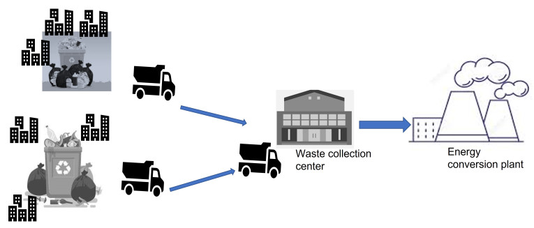
Effective surveillance during smart cities' sustainable development allows their cleanliness to be maintained by reusing waste to produce renewable energy. This study quantifies the biodegradable waste generated in specific regions of several cities and presents ways to convert it into renewable energy. This energy can then be used to partially support regional energy demands. This study explores ways of reducing carbon emissions for biodegradable waste collection processes in regional centers, ultimately sending the biodegradable waste to the energy conversion center. The smart production system allows for the flexible production and autonomation of rates of conversion; green technology depends on each regional center's research management, which is a decision variable for reducing carbon emissions. The major contribution of this study is to consider an energy supply chain management with flexibility of energy conversion under the reduction of carbon emissions, which leads to a sustainable ESCM with the global maximum profit. This study uses mathematical modeling to decrease biodegradable waste with conversion of energy through a classical optimization technique. The solution to this mathematical model yielded significant results, providing insight into waste reduction, reduced carbon emissions and the conversion of biodegradable waste to energy. The model is examined using numerical experiments, and its conclusion supports the model with the fundamental assumptions. Results of sensitivity analysis provide insight into the reduction and re-utilization of wastes, carbon emission reduction, and the benefits of using renewable energy.

| [1] |
A. S. Mahapatra, A. Dasgupta, A. K. Shaw, B. Sarkar, An inventory model with uncertain demand under preservation strategy for deteriorating items, RAIRO Oper. Res., 56 (2022), 4251–4280. https://doi.org/10.1051/ro/2022145 doi: 10.1051/ro/2022145

|
| [2] |
D. Yadav, R. Singh, A. Kumar, B. Sarkar, Reduction of pollution through sustainable and flexible production by controlling by-products, J. Environ. Inf., 40 (2022), 106–124. https://doi.org/10.3808/jei.202200476 doi: 10.3808/jei.202200476
|
| [3] |
B. Sarkar, J. Joo, Y. Kim, H. Park, M. Sarkar, Controlling defective items in a complex multi-phase manufacturing system, RAIRO Oper. Res., 56 (2022), 871–889. https://doi.org/10.1051/ro/2022019 doi: 10.1051/ro/2022019
|
| [4] |
A. S. Mahapatra, M. S. Mahapatra, B. Sarkar, S. K. Majumder, Benefit of preservation technology with promotion and time-dependent deterioration under fuzzy learning, Expert Syst. Appl., 201 (2022) 117169. https://doi.org/10.1016/j.eswa.2022.117169 doi: 10.1016/j.eswa.2022.117169
|
| [5] |
B. Sarkar, B. Ganguly, S. Pareek, L. E. Cárdenas-Barrón, A three-echelon green supply chain management for biodegradable products with three transportation modes, Comput. Ind. Eng., 174 (2022), 108727. https://doi.org/10.1016/j.cie.2022.108727 doi: 10.1016/j.cie.2022.108727
|
| [6] |
M. Sarkar, Y. W. Seo, Renewable energy supply chain management with flexibility and automation in a production system, J. Cleaner Prod., 324 (2021), 129149. https://doi.org/10.1016/j.jclepro.2021.129149 doi: 10.1016/j.jclepro.2021.129149
|
| [7] |
H. M. Wee, W. H. Yang, C. W. Chou, M. V. Padilan, Renewable energy supply chains, performance, application barriers, and strategies for further development, Renewable Sustainable Energy Rev., 16 (2012), 5451–5465. https://doi.org/10.1016/j.rser.2012.06.006 doi: 10.1016/j.rser.2012.06.006
|
| [8] |
I. D. Wangsa, T. M. Yang, H. M. Wee, The effect of price-dependent demand on the sustainable electrical energy supply chain, Energies, 11 (2018), 1645. https://doi.org/10.3390/en11071645 doi: 10.3390/en11071645
|
| [9] |
Y. Fernando, P. S. Bee, C. J. C. Jabbour, A. M. T. Thomé, Understanding the effects of energy management practices on renewable energy supply chains: Implications for energy policy in emerging economies, Energy Policy, 118 (2018), 418–428. https://doi.org/10.1016/j.enpol.2018.03.043 doi: 10.1016/j.enpol.2018.03.043
|
| [10] |
T. Mukherjee, I. Sangal, B. Sarkar, T. M. Alkadash, Mathematical estimation for maximum flow of goods within a cross-dock to reduce inventory, Math. Biosci. Eng., 19 (2022), 13710–13731. https://doi.org/10.3934/mbe.2022639 doi: 10.3934/mbe.2022639
|
| [11] |
B. Sarkar, D. Takeyeva, R. Guchhait, M. Sarkar, Optimized radio-frequency identification system for different warehouse shapes, Knowl. Based Syst., 258 (2022), 109811. https://doi.org/10.1016/j.knosys.2022.109811 doi: 10.1016/j.knosys.2022.109811
|
| [12] |
A. T. Hoang, P. S. Varbanov, S. Nižetić, R. Sirohi, A. Pandey, R. Luque, et al., Perspective review on Municipal Solid Waste-to-energy route: Characteristics, management strategy, and role in circular economy, J. Cleaner Prod., 359 (2022), 131897. https://doi.org/10.1016/j.jclepro.2022.131897 doi: 10.1016/j.jclepro.2022.131897
|
| [13] |
P. Alam, M. Sharholy, A. H. Khan, K. Ahmad, T. Alomayri, N. Radwan, A. Aziz, Energy generation and revenue potential from municipal solid waste using system dynamic approach, Chemosphere, 299 (2022), 134351. https://doi.org/10.1016/j.chemosphere.2022.134351 doi: 10.1016/j.chemosphere.2022.134351
|
| [14] |
S. Varjani, H. Shahbeig, K. Popat, Z. Patel, S. Vyas, A. V. Shah, D. Barceló, H. H. Ngo, C. Sonne, S. S. Lam, M. Aghbashlo, M. Tabatabaei, Sustainable management of municipal solid waste through waste-to-energy technologies, Bioresour. Technol., 355 (2022), 127247. https://doi.org/10.1016/j.biortech.2022.127247 doi: 10.1016/j.biortech.2022.127247
|
| [15] |
M. S. Habib, M. Omair, M. B. Ramzan, T. N. Chaudhary, M. Farooq, B. Sarkar, A robust possibilistic flexible programming approach toward a resilient and cost-efficient biodiesel supply chain network, J. Cleaner Prod., 366 (2022), 132752. https://doi.org/10.1016/j.jclepro.2022.132752 doi: 10.1016/j.jclepro.2022.132752
|
| [16] |
L. C. Malav, K. K. Yadav, N. Gupta, S. Kumar, G. K. Sharma, S. Krishnan, et al., A review on municipal solid waste as a renewable source for waste-to-energy project in India: Current practices, challenges, and future opportunities, J. Cleaner Prod., 277 (2020), 123227. https://doi.org/10.1016/j.jclepro.2020.123227 doi: 10.1016/j.jclepro.2020.123227
|
| [17] |
M. Mohammadi, I. Harjunkoski, Performance analysis of waste-to-energy technologies for sustainable energy generation in integrated supply chains, Comput. Chem. Eng., 140 (2020), 106905. https://doi.org/10.1016/j.compchemeng.2020.106905 doi: 10.1016/j.compchemeng.2020.106905
|
| [18] |
R. Zhao, L. Sun, X. Zou, M. Fujii, L. Dong, Y. Dou, et al., Towards a Zero Waste city-an analysis from the perspective of energy recovery and landfill reduction in Beijing, Energy, 223 (2021), 120055. https://doi.org/10.1016/j.energy.2021.120055 doi: 10.1016/j.energy.2021.120055
|
| [19] |
M. Sarkar, B. D. Chung, Flexible work-in-process production system in supply chain management under quality improvement, Int. J. Prod. Res., 58 (2020), 3821–3838. https://doi.org/10.1080/00207543.2019.1634851 doi: 10.1080/00207543.2019.1634851
|
| [20] |
A. S. H. Kugele, W. Ahmed, B. Sarkar, Geometric programming solution of second degree difficulty for carbon ejection controlled reliable smart production system, RAIRO Oper. Res., 56 (2022), 1013–1029. https://doi.org/10.1051/ro/2022028 doi: 10.1051/ro/2022028
|
| [21] |
B. Sarkar, B. K. Dey, M. Sarkar, S. J. Kim, A smart production system with an autonomation technology and dual channel retailing, Comput. Ind. Eng., 173 (2022), 108607. https://doi.org/10.1016/j.cie.2022.108607 doi: 10.1016/j.cie.2022.108607
|
| [22] |
A. K. Mondal, S. Pareek, K. Chaudhuri, A. Bera, R. K. Bachar, B. Sarkar, Technology license sharing strategy for remanufacturing industries under a closed-loop supply chain management bonding, RAIRO Oper. Res., 56 (2022), 3017–3045. https://doi.org/10.1051/ro/2022058 doi: 10.1051/ro/2022058
|
| [23] |
S. K. Hota, S. K. Ghosh, B. Sarkar, Involvement of smart technologies in an advanced supply chain management to solve unreliability under distribution robust approach, AIMS Environ. Sci., 9 (2022), 461–492. https://doi:10.3934/environsci.2022028 doi: 10.3934/environsci.2022028
|
| [24] | M. Sarkar, B. Sarkar, A. Dolgui, An automated smart production with system reliability under a leader-follower strategy of supply chain management, in IFIP International Conference on Advances in Production Management Systems, 663 (2022), 459–467. |
| [25] |
L. Čuček, P. S. Varbanov, J. J. Klemeš, Z. Kravanj, Total footprints-based multi-criteria optimisation of regional biomass energy supply chains, Energy, 44 (2012), 135–145. https://doi.org/10.1016/j.energy.2012.01.040 doi: 10.1016/j.energy.2012.01.040
|
| [26] |
Q. Bai, Y. Gong, M. Jin, X. Xu, Effects of carbon emission reduction on supply chain coordination with vendor-managed deteriorating product inventory, Int. J. Prod. Econ., 208 (2019), 83–99. https://doi.org/10.1016/j.ijpe.2018.11.008 doi: 10.1016/j.ijpe.2018.11.008
|
| [27] |
J. Yang, Z. Zhang, M. Hong, M. Yang, J. Chen, An oligarchy game model for the mobile waste heat recovery energy supply chain, Energy, 210 (2020), 118548. https://doi.org/10.1016/j.energy.2020.118548 doi: 10.1016/j.energy.2020.118548
|
| [28] |
S. Kumar, K. Sigroha, Meenu, K. Kumar, B. Sarkar, Manufacturing/remanufacturing based supply chain management under advertisements and carbon emissions process, RAIRO Oper. Res., 56 (2022), 831–851. https://doi.org/10.1051/ro/2021189 doi: 10.1051/ro/2021189
|
| [29] |
B. Sarkar, S. Kar, K. Basu, R. Guchhait, A sustainable managerial decision-making problem for a substitutable product in a dual-channel under carbon tax policy, Comput. Ind. Eng., 172 (2022), 108635. https://doi.org/10.1016/j.cie.2022.108635 doi: 10.1016/j.cie.2022.108635
|
| [30] |
B. Oryani, A. Moridian, B. Sarkar, S. Rezania, H. Kamyab, M. K. Khan, Assessing the financial resource curse hypothesis in Iran: The novel dynamic ARDL approach, Resour. Policy, 78 (2022), 102899. https://doi.org/10.1016/j.resourpol.2022.102899 doi: 10.1016/j.resourpol.2022.102899
|
| [31] |
B. Sarkar, B. Ganguly, S. Pareek, L. E. Cárdenas-Barrón, A three-echelon green supply chain management for biodegradable products with three transportation modes, Comput. Ind. Eng., 174 (2022), 108727. https://doi.org/10.1016/j.cie.2022.108727 doi: 10.1016/j.cie.2022.108727
|
| [32] |
R. K. Bachar, S. Bhuniya, S. K. Ghosh, A. AlArjani, E. Attia, M. S. Uddin, et al., Product outsourcing policy for a sustainable flexible manufacturing system with reworking and green investment, Math. Biosci. Eng., 20 (2023), 1376–1401. https://doi.org/10.3934/mbe.2023062 doi: 10.3934/mbe.2023062
|
| [33] |
G. Gallego, I. Moon, The distribution free newsboy problem: Review and extensions, J. Oper. Res. Soc., 44 (1993), 825–834. http://dx.doi.org/10.1057/jors.1993.141 doi: 10.1057/jors.1993.141
|

Figures(2) / Tables(5)

Mitali Sarkar, Yong Won Seo. Biodegradable waste to renewable energy conversion under a sustainable energy supply chain management[J]. Mathematical Biosciences and Engineering, 2023, 20(4): 6993-7019. doi: 10.3934/mbe.2023302


 DownLoad: