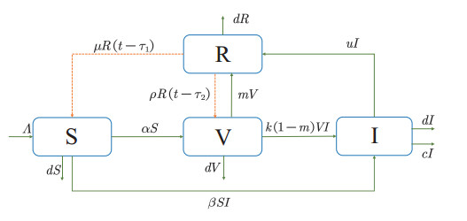
Since the outbreak of COVID-19, there has been widespread concern in the community, especially on the recent heated debate about when to get the booster vaccination. In order to explore the optimal time for receiving booster shots, here we construct an $ SVIR $ model with two time delays based on temporary immunity. Second, we theoretically analyze the existence and stability of equilibrium and further study the dynamic properties of Hopf bifurcation. Then, the statistical analysis is conducted to obtain two groups of parameters based on the official data, and numerical simulations are carried out to verify the theoretical analysis. As a result, we find that the equilibrium is locally asymptotically stable when the booster vaccination time is within the critical value. Moreover, the results of the simulations also exhibit globally stable properties, which might be more beneficial for controlling the outbreak. Finally, we propose the optimal time of booster vaccination and predict when the outbreak can be effectively controlled.
Citation: Zimeng Lv, Xinyu Liu, Yuting Ding. Dynamic behavior analysis of an $ SVIR $ epidemic model with two time delays associated with the COVID-19 booster vaccination time[J]. Mathematical Biosciences and Engineering, 2023, 20(4): 6030-6061. doi: 10.3934/mbe.2023261
Since the outbreak of COVID-19, there has been widespread concern in the community, especially on the recent heated debate about when to get the booster vaccination. In order to explore the optimal time for receiving booster shots, here we construct an $ SVIR $ model with two time delays based on temporary immunity. Second, we theoretically analyze the existence and stability of equilibrium and further study the dynamic properties of Hopf bifurcation. Then, the statistical analysis is conducted to obtain two groups of parameters based on the official data, and numerical simulations are carried out to verify the theoretical analysis. As a result, we find that the equilibrium is locally asymptotically stable when the booster vaccination time is within the critical value. Moreover, the results of the simulations also exhibit globally stable properties, which might be more beneficial for controlling the outbreak. Finally, we propose the optimal time of booster vaccination and predict when the outbreak can be effectively controlled.

| [1] |
N. Zhu, D. Zhang, W. Wang, X. Li, B. Yang, J. Song, et al., A novel coronavirus from patients with pneumonia in China, N. Engl. J. Med., 382 (2020), 727–733. https://doi.org/10.1056/NEJMoa2001017 doi: 10.1056/NEJMoa2001017

|
| [2] |
H. Zhang, F. Du, X. Cao, X. Feng, H. Zhang, Z. Wu, et al., Clinical characteristics of coronavirus disease 2019 (COVID-19) in patients out of Wuhan from China: a case control study, BMC Infect. Dis., 21 (2021), 207. https://doi.org/10.1186/s12879-021-05897-z doi: 10.1186/s12879-021-05897-z
|
| [3] |
C. Huang, Y. Wang, X. Li, L. Ren, J. Zhao, Y. Hu, et al., Clinical features of patients infected with 2019 novel coronavirus in Wuhan, China, Lancet, 395 (2020), 497–506. https://doi.org/10.1016/S0140-6736(20)30183-5 doi: 10.1016/S0140-6736(20)30183-5
|
| [4] |
M. A. Hassan, A. A. Bala, A. I. Jatau, Low rate of COVID-19 vaccination in Africa: a cause for concern, Ther. Adv. Vaccines Immun., 10 (2022), 1–3. https://doi.org/10.1177/25151355221088159 doi: 10.1177/25151355221088159
|
| [5] |
S. O. Minka, F. H. Minka, A tabulated summary of the evidence on humoral and cellular responses to the SARS-CoV-2 Omicron VOC, as well as vaccine efficacy against this variant, Immunol. Lett., 243 (2022), 38–43. https://doi.org/10.1016/j.imlet.2022.02.002 doi: 10.1016/j.imlet.2022.02.002
|
| [6] |
W. O. Kermack, A. G. Mckendrick, A contribution to the mathematical theory of epidemics, Proc. Roy. Soc., 115 (1927), 111–124. https://doi.org/10.1098/rspa.1927.0118 doi: 10.1098/rspa.1927.0118
|
| [7] |
A. Din, Y. Li, F. M. Khan, Z. U. Khan, P. Liu, On Analysis of fractional order mathematical model of Hepatitis B using Atangana Baleanu Caputo (ABC) derivative, Fractals, 30 (2022), 2240017. https://doi.org/10.1142/S0218348X22400175 doi: 10.1142/S0218348X22400175
|
| [8] |
B. Boukanjime, M. E. Fatini, A stochastic Hepatitis B epidemic model driven by Levy noise, Physica A, 521 (2019), 796–806. https://doi.org/10.1016/j.physa.2019.01.097 doi: 10.1016/j.physa.2019.01.097
|
| [9] |
Q. Liu, D. Jiang, T. Hayat, A. Alsaedi, Dynamical behavior of a stochastic epidemic model for cholera, J. Franklin Inst., 115 (1927), 111–124. https://doi.org/10.1016/j.jfranklin.2018.11.056 doi: 10.1016/j.jfranklin.2018.11.056
|
| [10] |
P. Liu, A. Din, Impact of information intervention on stochastic dengue epidemic model, Alex. Eng. J., 60 (2021), 5725–5739. https://doi.org/10.1016/j.aej.2021.03.068 doi: 10.1016/j.aej.2021.03.068
|
| [11] |
Z. Wang, G. Rost, S. M. Moghadas, Delay in booster schedule as a control parameter in vaccination dynamics, J. Math. Biol., 79 (2019), 2157–2182. https://doi.org/10.1007/s00285-019-01424-6 doi: 10.1007/s00285-019-01424-6
|
| [12] |
R. M. Anderson, B. T. Grenfell, Quantitative investigations of different vaccination policies for the control of congentila rubella syndrome (CRS) in the United Kingdom, Epidemiol. Infect., 96 (1986), 305–333. https://doi.org/10.1017/s0022172400066079 doi: 10.1017/s0022172400066079
|
| [13] |
M. E. Alexander, S. M. Moghadas, P. Rohani, A. R. Summers, Modelling the effect of a booster vaccination on disease epidemiology, J. Math. Biol., 52 (2006), 290–306. https://doi.org/10.1007/s00285-005-0356-0 doi: 10.1007/s00285-005-0356-0
|
| [14] |
T. Marinov, R. Marinova, Inverse problem for adaptive SIR model: Application to COVID-19 in Latin America, Infect. Dis. Modell., 7 (2022), 234–148. https://doi.org/10.1016/j.idm.2021.12.001 doi: 10.1016/j.idm.2021.12.001
|
| [15] |
H. Qiu, Q. Wang, Q. Wu, H. Zhou, Does flattening the curve make a difference? An investigation of the COVID-19 pandemic based on an SIR model, Int. Rev. Econ. Finance, 80 (2022), 159–165. https://doi.org/10.1016/j.iref.2022.02.063 doi: 10.1016/j.iref.2022.02.063
|
| [16] |
S. Annas, M. I. Pratama, M. Rifandi, W. Sanusi, S. Side, Stability analysis and numerical simulation of SEIR model for pandemic COVID-19 spread in Indonesia, Chaos Solitons Fractals, 139 (2020), 110072. https://doi.org/10.1016/j.chaos.2020.110072 doi: 10.1016/j.chaos.2020.110072
|
| [17] |
S. Paul, A. Mahata, U. Ghosh, B. Roy, Study of SEIR epidemic model and scenario analysis of COVID-19 pandemic, Ecol. Genet. Genom., 19 (2021), 100087. https://doi.org/10.1016/j.egg.2021.100087 doi: 10.1016/j.egg.2021.100087
|
| [18] |
D. Efimov, R. Ushirobira, On an interval prediction of COVID-19 development based on a SEIR epidemic model, Annu. Rev. Control, 51 (2021), 477–487. https://doi.org/10.1016/j.arcontrol.2021.01.006 doi: 10.1016/j.arcontrol.2021.01.006
|
| [19] |
Z. Chen, L. Feng, H. A. Lay Jr, K. Furati, A. Khaliq, SEIR model with unreported infected population and dynamic parameters for the spread of COVID-19, Math. Comput. Simul., 198 (2022), 31–46. https://doi.org/10.1016/j.matcom.2022.02.025 doi: 10.1016/j.matcom.2022.02.025
|
| [20] |
R. Li, Y. Song, H. Wang, G. Jiang, M. Xiao, Reactive diffusion epidemic model on human mobility networks: Analysis and applications to COVID-19 in China, Physica A, 609 (2023), 128337. https://doi.org/10.1016/j.physa.2022.128337 doi: 10.1016/j.physa.2022.128337
|
| [21] |
F. A. C. C. Chaluba, M. O. Souza, The SIR epidemic model from a PDE point of view, Math. Comput. Modell., 53 (2011), 1568–1574. https://doi.org/10.1016/j.mcm.2010.05.036 doi: 10.1016/j.mcm.2010.05.036
|
| [22] |
L. Bttcher, M. Xia, T. Chou, Why case fatality ratios can be misleading: individual and population based mortality estimates and factors influencing them, Phys. Biol., 17 (2020), 065003. https://doi.org/10.1088/1478-3975/ab9e59 doi: 10.1088/1478-3975/ab9e59
|
| [23] |
Q. Wu, X. Fan, H. Hong, Y. Gua, Z. Liu, S. Fang, Comprehensive assessment of side effects in COVID-19 drug pipeline from a network perspective, Food Chem. Toxicol., 145 (2020), e13476. https://doi.org/10.1016/j.fct.2020.111767 doi: 10.1016/j.fct.2020.111767
|
| [24] |
U. Tursen, B. Tursen, T. Lotti, Cutaneous side-effects of the potential COVID-19 drugs, Dermatol. Ther., 33 (2020), 31–46. https://doi.org/10.1111/dth.13476 doi: 10.1111/dth.13476
|
| [25] |
P. Wintachai, K. Prathom, Stability analysis of SEIR model related to efficiency of vaccines for COVID-19 situation, Heliyon, 7 (2021), e06812. https://doi.org/10.1016/j.heliyon.2021.e06812 doi: 10.1016/j.heliyon.2021.e06812
|
| [26] |
P. Jarumaneeroj, P. Dusadeerungsikul, T. Chotivanich, T. Nopsopon, K. Pongpirul, An epidemiology-based model for the operational allocation of COVID-19 vaccines: A case study of Thailand, Comput. Ind. Eng., 167 (2022), 108031. https://doi.org/10.1016/j.cie.2022.108031 doi: 10.1016/j.cie.2022.108031
|
| [27] |
L. Böher, J. Nagler, Decisive conditions for strategic vaccination against SARS-CoV-2, Chaos, 31 (2021), 101105. https://doi.org/10.1063/5.0066992 doi: 10.1063/5.0066992
|
| [28] |
A. Mahata, S. Paul, S. Mukherjee, B. Roy, Stability analysis and Hopf bifurcation in fractional order SEIRV epidemic model with a time delay in infected individuals, Partial Differ. Equations Appl. Math., 5 (2022), 100282. https://doi.org/10.1016/j.padiff.2022.100282 doi: 10.1016/j.padiff.2022.100282
|
| [29] |
H. Yang, Y. Wang, S. Kundu, Z. Song, Z. Zhang, Dynamics of an SIR epidemic model incorporating time delay and convex incidence rate, Results Phys., 32 (2022), 105025. https://doi.org/10.1016/j.rinp.2021.105025 doi: 10.1016/j.rinp.2021.105025
|
| [30] |
A. Khan, R. Ikram, A. Din, U. W. Humphries, A. Akgul, Stochastic COVID-19 SEIQ epidemic model with time-delay, Results Phys., 30 (2021), 104775. https://doi.org/10.1016/j.rinp.2021.104775 doi: 10.1016/j.rinp.2021.104775
|
| [31] |
C. Zhu, J. Zhu, Dynamic analysis of a delayed COVID-19 epidemic with home quarantine in temporal-spatial heterogeneous via global exponential attractor method, Chaos Solitons Fractals, 143 (2021), 110546. https://doi.org/10.1016/j.chaos.2020.110546 doi: 10.1016/j.chaos.2020.110546
|
| [32] |
E. M. Farah, S. Amine, K. Allali, Dynamics of a time-delayed two-strain epidemic model with general incidence rates, Chaos Solitons Fractals, 153 (2021), 111527. https://doi.org/10.1016/j.chaos.2021.111527 doi: 10.1016/j.chaos.2021.111527
|
| [33] |
H. Li, X. Liu, R. Yan, C. Liu, Hopf bifurcation analysis of a tumor virotherapy model with two time delays, Physica A, 553 (2020), 124266. https://doi.org/10.1016/j.physa.2020.124266 doi: 10.1016/j.physa.2020.124266
|
| [34] |
B. Sun, M. Li, F. Zhang, H. Wang, J. Liu, The characteristics and self-time-delay synchronization of two-time-delay complex Lorenz system, J. Franklin Inst., 356 (2019), 334–350. https://doi.org/10.1016/j.jfranklin.2018.09.031 doi: 10.1016/j.jfranklin.2018.09.031
|
| [35] |
M. Akio, S. Ferenc, Time delays and chaos in two competing species revisited, Appl. Math. Comput., 395 (2021), 125862. https://doi.org/10.1016/j.amc.2020.125862 doi: 10.1016/j.amc.2020.125862
|
| [36] |
H. Zhou, Z. Wang, D. Yuan, H. Song, Hopf bifurcation of a free boundary problem modeling tumor growth with angiogenesis and two time delays, Chaos Solitons Fractals, 153 (2021), 111578. https://doi.org/10.1016/j.chaos.2021.111578 doi: 10.1016/j.chaos.2021.111578
|
| [37] |
A. R. Hakimi, M. Azhdari, T. Binazadeh, Limit cycle oscillator in nonlinear systems with multiple time delays, Chaos Solitons Fractals, 153 (2021), 111454. https://doi.org/10.1016/j.chaos.2021.111454 doi: 10.1016/j.chaos.2021.111454
|
| [38] |
A. Adhikary, A. Pal, A six compartments with time-delay model SHIQRD for the COVID-19 pandemic in India: During lockdown and beyond, Alex. Eng. J., 61 (2022), 1403–1412. https://doi.org/10.1016/j.aej.2021.06.027 doi: 10.1016/j.aej.2021.06.027
|
| [39] |
A. Mahata, S. Paul, S. Mukherjee, B. Roy, Stability analysis and Hopf bifurcation in fractional order SEIRV epidemic model with a time delay in infected individuals, Partial Differ. Equations Appl. Math., 5 (2022), 100282. https://doi.org/10.1016/j.padiff.2022.100282 doi: 10.1016/j.padiff.2022.100282
|
| [40] |
Y. Zhang, J. Jia, Hopf bifurcation of an epidemic model with a nonlinear birth in population and vertical transmission, Appl. Math. Comput., 230 (2014), 164–173. https://doi.org/10.1016/j.amc.2013.12.084 doi: 10.1016/j.amc.2013.12.084
|
| [41] |
X. Duan, J. Yin, X. Li, Global Hopf bifurcation of an SIRS epidemic model with age-dependent recovery, Chaos Solitons Fractals, 104 (2017), 613–624. https://doi.org/10.1016/j.chaos.2017.09.029 doi: 10.1016/j.chaos.2017.09.029
|
| [42] |
Z. Zhang, S. Kundu, J. P. Tripathi, S. Bugalia, Stability and Hopf bifurcation analysis of an SVEIR epidemic model with vaccination and multiple time delays, Chaos Solitons Fractals, 131 (2020), 109483. https://doi.org/10.1016/j.chaos.2019.109483 doi: 10.1016/j.chaos.2019.109483
|
| [43] |
H. Yang, Y. Wang, S. Kundu, Z. Song, Z. Zhang, Dynamics of an SIR epidemic model incorporating time delay and convex incidence rate, Results Phys., 32 (2022), 105025. https://doi.org/10.1016/j.rinp.2021.105025 doi: 10.1016/j.rinp.2021.105025
|
| [44] |
Y. Ding, L. Zheng, Mathematical modeling and dynamics analysis of delayed nonlinear VOC emission system, Nonlinear Dyn., 109 (2022), 3157–3167. https://doi.org/10.1007/s11071-022-07532-1 doi: 10.1007/s11071-022-07532-1
|
| [45] |
Y. Ding, L. Zheng, J. Guo, Stability analysis of nonlinear glue flow system with delay, Math. Methods Appl. Sci., 45 (2022), 6861–6877. https://doi.org/10.1002/mma.8211 doi: 10.1002/mma.8211
|
| [46] |
Y. Song, Y. Peng, T. Zhang, The spatially inhomogeneous Hopf bifurcation induced by memory delay in a memory-based diffusion system, J. Differ. Equations, 300 (2021), 597–624. https://doi.org/10.1016/j.jde.2021.08.010 doi: 10.1016/j.jde.2021.08.010
|
| [47] |
Y. Song, H. Jiang, Y. Yuan, Turing-Hopf bifurcation in the reaction-diffusion system with delay and application to a diffusive predator-prey model, J. Appl. Anal. Comput., 9 (2019), 1132–1164. https://doi.org/10.1016/j.cnsns.2015.10.002 doi: 10.1016/j.cnsns.2015.10.002
|
| [48] |
I. Alam, A. Radovanovic, R. Incitti, A. A. Kamau, M. Alarawi, E. I. Azhar, et al., CovMT: an interactive SARS-CoV-2 mutation tracker, with a focus on critical variants, Lancet Infect. Dis., 21 (2021), 602. https://doi.org/10.1016/s1473-3099(21)00078-5 doi: 10.1016/s1473-3099(21)00078-5
|
| [49] |
T. Phan, Genetic diversity and evolution of SARS-CoV-2, Infect. Genet. Evol., 81 (2020), 104260. https://doi.org/10.1016/j.meegid.2020.104260 doi: 10.1016/j.meegid.2020.104260
|
| [50] |
M. Pachetti, B. Marini, F. Giudici, F. Benedetti, S. Angeletti, M. Ciccozzi, et al., Impact of lockdown on COVID-19 case fatality rate and viral mutations spread in 7 countries in europe and north america, J. Transl. Med., 18 (2020), 1–7. https://doi.org/10.1186/s12967-020-02501-x doi: 10.1186/s12967-020-02501-x
|
| [51] |
S. Y. Tartof, J. M. Slezak, H. Fischer, V. Hong, B. K. Ackerson, O. N. Ranasinghe, et al., Effectiveness of mRNA BNT162b2 COVID-19 vaccine up to 6 months in a large integrated health system in the USA: a retrospective cohort study, Lancet, 398 (2021), 1407–1416. https://doi.org/10.1016/S0140-6736(21)02183-8 doi: 10.1016/S0140-6736(21)02183-8
|
| [52] |
J. L. Bayart, J. Douxfils, C. Gillot, C. David, F. Mullier, M. Elsen, et al., Waning of IgG, total and neutralizing antibodies 6 months post-vaccination with BNT162b2 in healthcare workers, Vaccines, 9 (2021), 1092. https://doi.org/10.3390/vaccines9101092 doi: 10.3390/vaccines9101092
|
| [53] |
S. Liu, X. Yang, Y. Bia, Y. Li, Dynamic behavior and optimal scheduling for mixed vaccination strategy with temporary immunity, Discrete Contin. Dyn. Syst., 24 (2019), 1469–1483. https://doi.org/10.3934/dcdsb.2018216 doi: 10.3934/dcdsb.2018216
|
| [54] |
C. T. Ng, T. C. E. Heng, D. Tsadikovich, E. Levner, A. Elalouf, S. Hovav, A multi-criterion approach to optimal vaccination planning: Method and solution, Comput. Ind. Eng., 126 (2018), 637–649. https://doi.org/10.1016/j.cie.2018.10.018 doi: 10.1016/j.cie.2018.10.018
|
| [55] |
M. Xia, L. Böher, T. Chou, Controlling epidemics through optimal allocation of test kits and vaccine doses across networks, IEEE Trans. Network Sci. Eng., 9 (2022), 1422–1436. https://doi.org/10.1109/TNSE.2022.3144624 doi: 10.1109/TNSE.2022.3144624
|
| [56] |
Z. Lv, J. Zeng, Y. Ding, X. Liu, Stability analysis of time-delayed SAIR model for duration of vaccine in the context of temporary immunity for COVID-19 situation, Electron. Res. Arch., 31 (2023), 1004–1030. https://doi.org/10.3934/era.2023050 doi: 10.3934/era.2023050
|
Figures(11) / Tables(2)

Zimeng Lv, Xinyu Liu, Yuting Ding. Dynamic behavior analysis of an $ SVIR $ epidemic model with two time delays associated with the COVID-19 booster vaccination time[J]. Mathematical Biosciences and Engineering, 2023, 20(4): 6030-6061. doi: 10.3934/mbe.2023261


 DownLoad: