Mathematical modeling and stability analysis of the time-delayed $ SAIM $ model for COVID-19 vaccination and media coverage

Xinyu Liu; Zimeng Lv; Yuting Ding; Xinyu Liu; Zimeng Lv; Yuting Ding

doi:10.3934/mbe.2022294

Mathematical Biosciences and Engineering

2022, Volume 19, Issue 6: 6296-6316. doi: 10.3934/mbe.2022294

Previous Article Next Article

Research article

Mathematical modeling and stability analysis of the time-delayed $ SAIM $ model for COVID-19 vaccination and media coverage

Department of Mathematics, Northeast Forestry University, Harbin 150040, China

Received: 29 January 2022 Revised: 31 March 2022 Accepted: 31 March 2022 Published: 19 April 2022

Since the COVID-19 outbreak began in early 2020, it has spread rapidly and threatened public health worldwide. Vaccination is an effective way to control the epidemic. In this paper, we model a $ SAIM $ equation. Our model involves vaccination and the time delay for people to change their willingness to be vaccinated, which is influenced by media coverage. Second, we theoretically analyze the existence and stability of the equilibria of our model. Then, we study the existence of Hopf bifurcation related to the two equilibria and obtain the normal form near the Hopf bifurcating critical point. Third, numerical simulations based two groups of values for model parameters are carried out to verify our theoretical analysis and assess features such as stable equilibria and periodic solutions. To ensure the appropriateness of model parameters, we conduct a mathematical analysis of official data. Next, we study the effect of the media influence rate and attenuation rate of media coverage on vaccination and epidemic control. The analysis results are consistent with real-world conditions. Finally, we present conclusions and suggestions related to the impact of media coverage on vaccination and epidemic control.
- COVID-19 epidemic,
- media coverage,
- vaccination,
- time-delay,
- Hopf bifurcation,
- normal form,
- multiple time scales method
Citation: Xinyu Liu, Zimeng Lv, Yuting Ding. Mathematical modeling and stability analysis of the time-delayed $ SAIM $ model for COVID-19 vaccination and media coverage[J]. Mathematical Biosciences and Engineering, 2022, 19(6): 6296-6316. doi: 10.3934/mbe.2022294

Related Papers:

Abstract

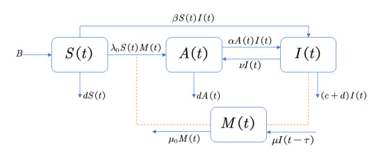
Since the COVID-19 outbreak began in early 2020, it has spread rapidly and threatened public health worldwide. Vaccination is an effective way to control the epidemic. In this paper, we model a $ SAIM $ equation. Our model involves vaccination and the time delay for people to change their willingness to be vaccinated, which is influenced by media coverage. Second, we theoretically analyze the existence and stability of the equilibria of our model. Then, we study the existence of Hopf bifurcation related to the two equilibria and obtain the normal form near the Hopf bifurcating critical point. Third, numerical simulations based two groups of values for model parameters are carried out to verify our theoretical analysis and assess features such as stable equilibria and periodic solutions. To ensure the appropriateness of model parameters, we conduct a mathematical analysis of official data. Next, we study the effect of the media influence rate and attenuation rate of media coverage on vaccination and epidemic control. The analysis results are consistent with real-world conditions. Finally, we present conclusions and suggestions related to the impact of media coverage on vaccination and epidemic control.

References

[1]	H. Guliyev, Determining the spatial effects of COVID-19 using the spatial panel data model, Spatial Stat., 38 (2020), 100443. https://doi.org/10.1016/j.spasta.2020.100443 doi: 10.1016/j.spasta.2020.100443
[2]	Y. Niu, J. Rui, Q. Wang, W. Zhang, Z. Chen, F. Xie, et al., Containing the transmission of COVID-19: a modeling study in 160 countries, Front. Med., 8 (2021), 701836. https://doi.org/10.3389/fmed.2021.701836 doi: 10.3389/fmed.2021.701836
[3]	M. Habadi, T. H. Balla Abdalla, N. Hamza, A. Al-Gedeei, COVID-19 Reinfection, Cureus, 13 (2021), e12730. https://dx.doi.org/10.7759%2Fcureus.12730
[4]	S. R. Kannan, A. N. Spratt, A. R. Cohen, S. H. Naqvi, H. S. Chand, T. P. Quinn, et al., Evolutionary analysis of the Delta and Delta plus variants of the SARS-CoV-2 viruses, J. Autoimmun., 124 (2021), 102715. https://doi.org/10.1016/j.jaut.2021.102715 doi: 10.1016/j.jaut.2021.102715
[5]	F. Wei, R. Xue, Stability and extinction of SEIR epidemic models with generalized nonlinear incidence, Math. Comput. Simul., 170 (2020), 1–15. https://doi.org/10.1016/j.matcom.2018.09.029 doi: 10.1016/j.matcom.2018.09.029
[6]	O. Khyar, K. Allali, Global dynamics of a multi-strain SEIR epidemic model with general incidence rates: application to COVID-19 pandemic, Nonlinear Dyn., 102 (2020), 489–509. https://doi.org/10.1007/s11071-020-05929-4 doi: 10.1007/s11071-020-05929-4
[7]	Z. Zhang, A. Zeb, O. F. Egbelowo, V. S. Erturk, Dynamics of a fractional order mathematical model for COVID-19 epidemic, Adv. Differ. Equations, 2020 (2020), 420. https://doi.org/10.1186/s13662-020-02873-w doi: 10.1186/s13662-020-02873-w
[8]	S. Annas, M. I. Pratama, M. Rifandi, W. Sanusi, S. Side, Stability analysis and numerical simulation of SEIR model for pandemic COVID-19 spread in Indonesia, Chaos Soliton Fract., 139 (2020), 110072. https://doi.org/10.1016/j.chaos.2020.110072 doi: 10.1016/j.chaos.2020.110072
[9]	H. M. Youssef, N. A. Alghamdi, M. A. Ezzat, A. A. El-Bary, A. M. Shawky, A new dynamical modeling SEIR with global analysis applied to the real data of spreading COVID-19 in Saudi Arabia, Math. Biosci. Eng., 17 (2020), 7018–7044. https://doi.org/10.3934/mbe.2020362 doi: 10.3934/mbe.2020362
[10]	M. Abdy, S. Side, S. Annas, W. Nur, W. Sanusi, An SIR epidemic model for COVID-19 spread with fuzzy parameter: the case of Indonesia, Adv. Differ. Equations, 2021 (2021), 105. https://doi.org/10.1186/s13662-021-03263-6 doi: 10.1186/s13662-021-03263-6
[11]	L. Wang, Z. Liu, X. Zhang, Global dynamics for an age-structured epidemic model with media impact and incomplete vaccination, Nonlinear Anal., 32 (2016), 136–158. https://doi.org/10.1016/j.nonrwa.2016.04.009 doi: 10.1016/j.nonrwa.2016.04.009
[12]	C. Z. Olorunsaiye, K. K. Yusuf, K. Reinhart, H. M. Salihu, COVID-19 and child vaccination: a systematic approach to closing the immunization gap, Int. J. Matern. Child Health Aids, 9 (2020), 381–385. http://orcid.org/0000-0003-4725-0448
[13]	R. M. Anderson, R. M. May, Vaccination and herd immunity to infectious diseases, Nature, 318 (1985), 323–329. https://doi.org/10.1038/318323a0 doi: 10.1038/318323a0
[14]	S. Zhai, G. Luo, T. Huang, X. Wang, J. Tao, P. Zhou, Vaccination control of an epidemic model with time delay and its application to COVID-19, Nonlinear Dyn., 106 (2021), 1279–1292. https://doi.org/10.1007/s11071-021-06533-w doi: 10.1007/s11071-021-06533-w
[15]	J. Yang, Q. Zhang, Z. Cao, J. Gao, D. Pfeiffer, L. Zhong, et al., The impact of non-pharmaceutical interventions on the prevention and control of COVID-19 in New York City, Chaos, 31 (2021), 021101. https://doi.org/10.1101/2020.12.01.20242347 doi: 10.1101/2020.12.01.20242347
[16]	G. O. Agaba, Y. N. Kyrychko, K. B. Blyuss, Dynamics of vaccination in a time-delayed epidemic model with awareness, Math. Biosci., 294 (2017), 92–99. https://doi.org/10.1016/j.mbs.2017.09.007 doi: 10.1016/j.mbs.2017.09.007
[17]	I. Z. Kiss, J. Cassell, M. Recker, P. L. Simon, The impact of information transmission on epidemic outbreaks, Math. Biosco., 225 (2010), 1–10. https://doi.org/10.1016/j.mbs.2009.11.009 doi: 10.1016/j.mbs.2009.11.009
[18]	T. K. Kar, S. K. Nandi, S. Jana, M. Mandal, Stability and bifurcation analysis of an epidemic model with the effect of media, Chaos Soliton Fract., 120 (2019), 188–199. https://doi.org/10.1016/j.chaos.2019.01.025 doi: 10.1016/j.chaos.2019.01.025
[19]	Z. Liu, P. Magal, O. Seydi, G. Webb, A COVID-19 epidemic model with latency period, Infect. Dis. Model., 5 (2020), 323–337. https://doi.org/10.1016/j.idm.2020.03.003 doi: 10.1016/j.idm.2020.03.003
[20]	C. C. McCluskey, Global stability for an SIR epidemic model with delay and nonlinear incidence, Nonlinear Anal., 11 (2010), 3106–3109. https://doi.org/10.1016/j.nonrwa.2009.11.005 doi: 10.1016/j.nonrwa.2009.11.005
[21]	X. Zhou, J. Cui, Stability and Hopf bifurcation of a delay eco-epidemiological model with nonlinear incidence rate, Math. Model. Anal., 15 (2010), 547–569. https://doi.org/10.3846/1392-6292.2010.15.547-569 doi: 10.3846/1392-6292.2010.15.547-569
[22]	X. Zhou, Z. Guo, Analysis of stability and Hopf bifurcation for an eco-epidemiological model with distributed delay, Electron. J. Qual. Theory, 44 (2012), 1–22. https://doi.org/10.14232/ejqtde.2012.1.44 doi: 10.14232/ejqtde.2012.1.44
[23]	W. B. Ma, S. Mei, Y. Takeuchi, Global stability of an SIR epidemic model with time delay, Appl. Math. Lett., 17 (2003), 1141–1145. https://doi.org/10.1016/j.aml.2003.11.005 doi: 10.1016/j.aml.2003.11.005
[24]	A. K. Misra, A. Sharma, V. Singh, Effect of awareness programs in controlling the prevalence of an epidemic with time delay, J. Biol. Syst., 19 (2011), 389–402. https://doi.org/10.1142/S0218339011004020 doi: 10.1142/S0218339011004020
[25]	M. J. Mulligan, An inactivated virus candidate vaccine to prevent COVID-19, J. Am. Med. Assoc., 324 (2020), 943–945. http://jamanetwork.com/article.aspx?doi = 10.1001/jama.2020.15539
[26]	S. Rahman, M. M. Rahman, M. Rahman, M. N. Begum, M. Sarmin, M. Mahfuz, et al., COVID-19 reinfections among naturally infected and vaccinated individuals, Sci. Rep., 12 (2022), 1438. https://doi.org/10.1038/s41598-022-05325-5 doi: 10.1038/s41598-022-05325-5

Reader Comments

Your name:*

Email:*
© 2022 the Author(s), licensee AIMS Press. This is an open access article distributed under the terms of the Creative Commons Attribution License (http://creativecommons.org/licenses/by/4.0)