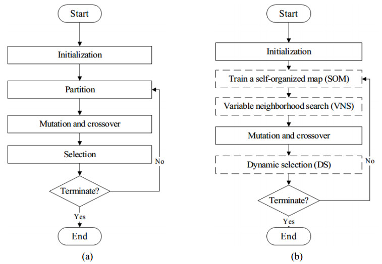
Many real-world problems can be classified as multimodal optimization problems (MMOPs), which require to locate global optima as more as possible and refine the accuracy of found optima as high as possible. When dealing with MMOPs, how to divide population and obtain effective niches is a key to balance population diversity and convergence during evolution. In this paper, a self-organizing map (SOM) based differential evolution with dynamic selection strategy (SOMDE-DS) is proposed to improve the performance of differential evolution (DE) in solving MMOPs. Firstly, a SOM based method is introduced as a niching technique to divide population reasonably by using the similarity information among different individuals. Secondly, a variable neighborhood search (VNS) strategy is proposed to locate more possible optimal regions by expanding the search space. Thirdly, a dynamic selection (DS) strategy is designed to balance exploration and exploitation of the population by taking advantages of both local search strategy and global search strategy. The proposed SOMDE-DS is compared with several widely used multimodal optimization algorithms on benchmark CEC'2013. The experimental results show that SOMDE-DS is superior or competitive with the compared algorithms.
Citation: Shihao Yuan, Hong Zhao, Jing Liu, Binjie Song. Self-organizing map based differential evolution with dynamic selection strategy for multimodal optimization problems[J]. Mathematical Biosciences and Engineering, 2022, 19(6): 5968-5997. doi: 10.3934/mbe.2022279
Many real-world problems can be classified as multimodal optimization problems (MMOPs), which require to locate global optima as more as possible and refine the accuracy of found optima as high as possible. When dealing with MMOPs, how to divide population and obtain effective niches is a key to balance population diversity and convergence during evolution. In this paper, a self-organizing map (SOM) based differential evolution with dynamic selection strategy (SOMDE-DS) is proposed to improve the performance of differential evolution (DE) in solving MMOPs. Firstly, a SOM based method is introduced as a niching technique to divide population reasonably by using the similarity information among different individuals. Secondly, a variable neighborhood search (VNS) strategy is proposed to locate more possible optimal regions by expanding the search space. Thirdly, a dynamic selection (DS) strategy is designed to balance exploration and exploitation of the population by taking advantages of both local search strategy and global search strategy. The proposed SOMDE-DS is compared with several widely used multimodal optimization algorithms on benchmark CEC'2013. The experimental results show that SOMDE-DS is superior or competitive with the compared algorithms.

| [1] |
R. Tanabe, H. Ishibuchi, A review of evolutionary multimodal multiobjective optimization, IEEE Trans. Evol. Comput., 24 (2020), 193-200. https://doi.org/10.1109/TEVC.2019.2909744 doi: 10.1109/TEVC.2019.2909744

|
| [2] |
D. Chen, Y. Li, A development on multimodal optimization technique and its application in structural damage detection, Appl. Soft Comput., 91 (2020), 106264. https://doi.org/10.1016/j.asoc.2020.106264 doi: 10.1016/j.asoc.2020.106264
|
| [3] |
K. Wang, J. Zheng, F. Lu, H. Gao, A. Palanisamy, S. Zhuang, Varied-line-spacing switchable holographic grating using polymer-dispersed liquid crystal, Appl. Opt., 55 (2016), 4952-4957. https://doi.org/10.1364/AO.55.004952 doi: 10.1364/AO.55.004952
|
| [4] | A. W. Senior, R. Evans, J. Jumper, J. Kirkpatrick, L. Sifre, T. Green, et al., Improved protein structure prediction using potentials from deep learning, Nature, 577 (2020), 706-710. https://doi.org/10.1038/s41586-019-1923-7 |
| [5] |
J. Zhang, G. Ding, Y. Zou, S. Qin, J. Fu, Review of job shop scheduling research and its new perspectives under Industry 4.0, J. Intell. Manuf., 30 (2019), 1809-1830. https://doi.org/10.1007/s10845-017-1350-2 doi: 10.1007/s10845-017-1350-2
|
| [6] | A. Lambora, K. Gupta, K. Chopra, Genetic algorithm—a literature review, in 2019 International Conference on Machine Learning, Big Data, Cloud and Parallel Computing, 2019. https://doi.org/10.1109/COMITCon.2019.8862255 |
| [7] |
Bilal, M. Pant, H. Zaheer, L. Garcia-Hernandez, A. Abraham, Differential Evolution: a review of more than two decades of research, Eng. Appl. Artif. Intell., 90 (2020), 103479. https://doi.org/10.1016/j.engappai.2020.103479 doi: 10.1016/j.engappai.2020.103479
|
| [8] | H. Zhao, Z. H. Zhan, Y. Lin, X. F. Chen, X. N. Luo, J. Zhang, et al., Local binary pattern based adaptive differential evolution for multimodal optimization problems, IEEE Trans. Cybern., 50 (2020), 3343-3357. https://doi.org/10.1109/TCYB.2019.2927780 |
| [9] | H. Zhao, Z. H. Zhan, J. Zhang, Adaptive guidance-based differential evolution with archive strategy for multimodal optimization problems, in Proceedings IEEE Congress on Evolutionary Computation, (2020), 1-8. https://doi.org/10.1109/CEC48606.2020.9185582 |
| [10] | K. E. Parsopoulos, M. N. Vrahatis, Unified particle swarm optimization for solving constrained engineering optimization problems, in Advances in Natural Computation (eds. L. Wang, K. Chen, and Y. S. Ong), Springer Berlin Heidelberg, (2005), 582-591. https://doi.org/10.1007/11539902_71 |
| [11] | J. Liang, S. Ge, B. Y. Qu, K. Yu, F. Liu, H. Yang, et al., Classified perturbation mutation based particle swarm optimization algorithm for parameters extraction of photovoltaic models, Energy Convers. Manag., 203 (2020), 112138. https://doi.org/10.1016/j.enconman.2019.112138 |
| [12] | H. X. Chen, D. L. Fan, F. Lu, W. J. Huang, J. M. Huang, C. H. Cao, et al., Particle swarm optimization algorithm with mutation operator for particle filter noise reduction in mechanical fault diagnosis, Int. J. Pattern Recognit. Artif. Intell., 34 (2020), 2058012. https://doi.org/10.1142/S0218001420580124 |
| [13] |
X. F. Song, Y. Zhang, Y. N. Guo, X. Y. Sun, Y. L. Wang, Variable-size cooperative coevolutionary particle swarm optimization for feature selection on high-dimensional data, IEEE Trans. Evol. Comput., 24 (2020), 882-895. https://doi.org/10.1109/TEVC.2020.2968743 doi: 10.1109/TEVC.2020.2968743
|
| [14] | L. Qing, W. Gang, Y. Zaiyue, W. Qiuping, Crowding clustering genetic algorithm for multimodal function optimization, Appl. Soft Comput., 8 (2008), 88-95. https://10.1016/j.asoc.2006.10.014 |
| [15] |
B. Y. Qu, P. N. Suganthan, S. Das, A distance-based locally informed particle swarm model for multimodal optimization, IEEE Trans. Evol. Comput., 17 (2013), 387-402. https://doi.org/10.1109/TEVC.2012.2203138 doi: 10.1109/TEVC.2012.2203138
|
| [16] | Z. J. Wang, Z. H. Zhan, Y. Lin, W. J. Wu, H. Q. Yuan, T. L. Gu, et al., Dual-strategy differential evolution with affinity propagation clustering for multimodal optimization problems, IEEE Trans. Evol. Comput., 22 (2018), 894-908. https://doi.org/10.1109/TEVC.2017.2769108 |
| [17] | T. Kohonen, Self-organized formation of topologically correct feature maps, Biol. Cybern., 43 (1982). https://doi.org/10.1007/BF00337288 |
| [18] | T. Kohonen, Essentials of the self-organizing map, Neural Networks, 37 (2013), 52-65. https://doi.org/10.1016/j.neunet.2012.09.018 |
| [19] |
R. Storn, K. Price, Differential evolution—a simple and efficient heuristic for global optimization over continuous spaces, J. Glob. Optim., 11 (1997), 341-359, https://doi.org/10.1023/A:1008202821328 doi: 10.1023/A:1008202821328
|
| [20] |
B. Xue, M. Zhang, W. N. Browne, X. Yao, A survey on evolutionary computation approaches to feature selection, IEEE Trans. Evol. Comput., 20 (2016), 606-626. https://doi.org/10.1109/TEVC.2015.2504420 doi: 10.1109/TEVC.2015.2504420
|
| [21] | H. Bersini, M. Dorigo, S. Langerman, G. Seront, L. Gambardella, Results of the first international contest on evolutionary optimisation, in Proceedings of IEEE International Conference on Evolutionary Computation, (1996), 611-615. https://doi.org/10.1109/ICEC.1996.542670 |
| [22] | S. M. Guo, J. S. H. Tsai, C. C. Yang, T. H. Hsu, A self-organizing approach for L-SHADE incorporated with eigenvector-based crossover and successful-parent-selecting framework on CEC 2015 benchmark set, in Proceedings IEEE Congress on Evolutionary Computation, (2015), 1003-1010. https://doi.org/10.1109/CEC.2015.7256999 |
| [23] | N. Awad, M. Ali, P. Suganthan, R. Reynolds, An ensemble sinusoidal parameter adaptation incorporated with L-SHade for solving CEC2014 benchmark problems, in Proceedings IEEE Congress on Evolutionary Computation, (2016), 2958-2965. https://doi.org/10.1109/CEC.2016.7744163 |
| [24] | R. Tanabe, A. Fukunaga, Improving the search performance of SHADE using linear population size reduction, in Proceedings IEEE Congress on Evolutionary Computation, (2014), 1658-1665. https://doi.org/0.1109/CEC.2014.6900380 |
| [25] | N. Awad, M. Ali, P. Suganthan, Ensemble sinusoidal differential covariance matrix adaptation with Euclidean neighborhood for solving CEC2017 benchmark problems, in Proceedings IEEE Congress on Evolutionary Computation, (2017), 372-379. https://doi.org/10.1109/CEC.2017.7969336 |
| [26] | S. Akhmedova, V. Stanovov, E. Senmenkin, LSHADE algorithm with a rank-based selective pressure strategy for the circular antenna array design problem, in International Conference on Informatics in Control, Automation and Robotics, (2018), 159-165. https://doi.org/10.5220/0006852501590165 |
| [27] |
J. Brest, S. Greiner, B. Boskovic, M. Mernik, V. Zumer, Self-adapting control parameters in differential evolution: a comparative study on numerical benchmark problems, IEEE Trans. Evol. Comput., 10 (2006), 646-657. https://doi.org/10.1109/TEVC.2006.872133 doi: 10.1109/TEVC.2006.872133
|
| [28] | X. Rui, D. Wunsch, Survey of clustering algorithms, IEEE Trans. Neural Networks, 16 (2005), 645-678. https://doi.org/10.1109/TNN.2005.845141 |
| [29] |
T. Kanungo, D. M. Mount, N. S. Netanyahu, C. D. Piatko, R. Silverman, A. Y. Wu, An efficient k-means clustering algorithm: analysis and implementation, IEEE Trans. Pattern Anal. Mach. Intell., 24 (2002), 881-892. https://doi.org/10.1109/TPAMI.2002.1017616 doi: 10.1109/TPAMI.2002.1017616
|
| [30] |
B. Y. Qu, C. Li, J. Liang, L. Yan, K. Yu, Y. Zhu, A self-organized speciation based multi-objective particle swarm optimizer for multimodal multi-objective problems, Appl. Soft Comput., 86 (2020), 105886. https://doi.org/10.1016/j.asoc.2019.105886 doi: 10.1016/j.asoc.2019.105886
|
| [31] | Y. Hu, j. Wang, J. Liang, K. Yu, H. Song, Q. GUO, et al., A self-organizing multimodal multi-objective pigeon-inspired optimization algorithm, Sci. China Inf. Sci., 62 (2019), 70206. https://doi.org/10.1007/s11432-018-9754-6 |
| [32] |
H. Zhang, A. Zhou, S. Song, Q. Zhang, X. Z. Gao, J. Zhang, A self-organizing multiobjective evolutionary algorithm, IEEE Trans. Evol. Comput., 20 (2016), 792-806. https://doi.org/10.1109/TEVC.2016.2521868 doi: 10.1109/TEVC.2016.2521868
|
| [33] |
A. M. Kashtiban, S. Khanmohammadi, A genetic algorithm with SOM neural network clustering for multimodal function optimization, J. Intell. Fuzzy Syst., 35 (2018), 4543-4556. https://doi.org/10.3233/JIFS-131344 doi: 10.3233/JIFS-131344
|
| [34] | K. Zielinski, R. Laur, Stopping criteria for differential evolution in constrained single-objective optimization, in Advances in Differential Evolution, (eds. U. K. Chakraborty), Springer Berlin Heidelberg, (2008), 111-138. https://doi.org/10.1007/978-3-540-68830-3_4 |
| [35] | Q. Yang, W. N. Chen, Z. Yu, T. Gu, Y. Li, H. Zhang, J.Zhang, et al., Adaptive multimodal continuous ant colony optimization, IEEE Trans. Evol. Comput., 21 (2017), 191-205. https://doi.org/10.1109/TEVC.2016.2591064 |
| [36] | A. Hackl, C. Magele, W. Renhart, Extended firefly algorithm for multimodal optimization, in Proceedings 19th International Symposium on Electrical Apparatus and Technologies, (2016), 1-4. https://doi.org/10.1109/SIELA.2016.7543010 |
| [37] | R. Thomsen, Multimodal optimization using crowding-based differential evolution, in Proceedings of the 2004 Congress on Evolutionary Computation, (2004), 1382-1389. https://doi.org/10.1109/CEC.2004.1331058 |
| [38] | A. Petrowski, A clearing procedure as a niching method for genetic algorithms, in Proceedings of IEEE International Conference on Evolutionary Computation, (1996), 798-803. https://doi.org/10.1109/ICEC.1996.542703 |
| [39] |
B. Y. Qu, P. N. Suganthan, J. J. Liang, Differential evolution with neighborhood mutation for multimodal optimization, IEEE Trans. Evol. Comput., 16 (2012), 601-614. https://doi.org/10.1109/TEVC.2011.2161873 doi: 10.1109/TEVC.2011.2161873
|
| [40] |
X. Li, Niching without niching parameters: particle swarm optimization using a ring topology, IEEE Trans. Evol. Comput., 14 (2010), 150-169. https://https://doi.org/10.1109/TEVC.2009.2026270 doi: 10.1109/TEVC.2009.2026270
|
| [41] |
Z. Wei, W. Gao, G. Li, Q. Zhang, A penalty-based differential evolution for multimodal optimization, IEEE Trans. Cybern., 2021 (2021). https://doi.org/10.1109/TCYB.2021.3117359 doi: 10.1109/TCYB.2021.3117359
|
| [42] |
X. Lin, W. Luo, P. Xu, Differential evolution for multimodal optimization with species by nearest-better clustering, IEEE Trans. Cybern., 51 (2021), 970-983. https://doi.org/10.1109/TCYB.2019.2907657 doi: 10.1109/TCYB.2019.2907657
|
| [43] | Z. J. Wang, Z. H. Zhan, Y. Lin, W. J. Yu, H. Wang, S. Kwong, J. Zhang, et al., Automatic niching differential evolution with contour prediction approach for multimodal optimization problems, IEEE Trans. Evol. Comput., 24 (2020), 114-128. https://doi.org/10.1109/TEVC.2019.2910721 |
| [44] | X. Zhuoran, M. Polojärvi, M. Yamamoto, M. Furukawa, Attraction basin estimating GA: an adaptive and efficient technique for multimodal optimization, in Proceedings IEEE Congress on Evolutionary Computation, (2013), 333-340. https://doi.org/10.1109/CEC.2013.6557588 |
| [45] |
J. Liang, K. Qiao, T. Y. Cai, K. Yu, A clustering-based differential evolution algorithm for solving multimodal multi-objective optimization problems, Swarm Evol. Comput., 60 (2021), 100788. https://doi.org/10.1016/j.swevo.2020.100788 doi: 10.1016/j.swevo.2020.100788
|
| [46] |
Z. Hu, T. Zhou, Q. Su, M. Liu, A niching backtracking search algorithm with adaptive local search for multimodal multiobjective optimization, Swarm Evol. Comput., 69 (2022), 101031. https://doi.org/10.1016/j.swevo.2022.101031 doi: 10.1016/j.swevo.2022.101031
|
| [47] | M. G. Epitropakis, V. P. Plagianakos, M. N. Vrahatis, Finding multiple global optima exploiting differential evolution's niching capability, in Proceedings IEEE Symposium on Differential Evolution, (2011), 1-8. https://doi.org/10.1109/SDE.2011.5952058 |
| [48] | M. G. Epitropakis, X. Li, E. K. Burke, A dynamic archive niching differential evolution algorithm for multimodal optimization, in Proceedings IEEE Congress on Evolutionary Computation, (2013), 79-86. https://doi.org/10.1109/CEC.2013.6557556 |
| [49] | J. Wang, Enhancing particle swarm algorithm for multimodal optimization problems, in Proceedings International Conference on Computing Intelligence and Information System, (2017), 1-6. https://doi.org/10.1109/CIIS.2017.10 |
| [50] | W. Liu, L. Liu, T. Zhang, J. Liu, Multimodal function optimization based on improved ABC algorithm, in Proceedings 9th International Symposium on Computational Intelligence and Design, (2016), 246-249. https://doi.org/10.1109/ISCID.2016.1063 |
| [51] |
R. Cheng, M. Li, K. Li, X. Yao, Evolutionary multiobjective optimization-based multimodal optimization: fitness landscape approximation and peak detection, IEEE Trans. Evol. Comput., 22 (2018), 692-706. https://doi.org/10.1109/TEVC.2017.2744328 doi: 10.1109/TEVC.2017.2744328
|
| [52] |
Y. Wang, H. Li, G. G. Yen, W. Song, MOMMOP: multiobjective optimization for locating multiple optimal solutions of multimodal optimization problems, IEEE Trans. Cybern., 45 (2015), 830-843. https://doi.org/10.1109/TCYB.2014.2337117 doi: 10.1109/TCYB.2014.2337117
|
| [53] |
W. J. Yu, J. Y. Ji, Y. J. Gong, Q. Yang, J. Zhang, A tri-objective differential evolution approach for multimodal optimization, Inf. Sci., 423 (2018), 1-23. https://doi.org/10.1016/j.ins.2017.09.044 doi: 10.1016/j.ins.2017.09.044
|
| [54] | V. Steinhoff, P. Kerschke, P. Aspar, H. Trautmann, C. Grimme, Multiobjectivization of local search: single-objective optimization benefits from multi-objective gradient descent, in Proceedings IEEE Symposium Series on Computational Intelligence, (2020), 2445-2452. https://doi.org/10.1109/SSCI47803.2020.9308259 |
| [55] | P. Aspar, P. Kerschke, V. Steinhoff, H. Trautmann, C. Grimme, Multi3: optimizing multimodal single-objective continuous problems in the multi-objective space by means of multiobjectivization, in Evolutionary Multi-Criterion Optimization (eds. H. Ishibuchi, et al.), (2021), 12654. https://doi.org/10.1007/978-3-030-72062-9_25 |
| [56] | C. Grimme, P. Kerschke, P. Aspar, H. Trautmann, M. Preuss, A. Deutz, et al., Peeking beyond peaks: challenges and research potentials of continuous multimodal multi-objective optimization, Comput. Oper. Res., 136 (2021), 105489. https://doi.org/10.1016/j.cor.2021.105489 |
| [57] | X. Li, A. Engelbrecht, M. G. Epitropakis, Benchmark functions for CEC'2013 special session and competition on niching methods for multimodal function optimization. Available from: https://www.epitropakis.co.uk/sites/default/files/pubs/cec2013-niching-benchmark-tech-report.pdf. |
| [58] | W. Luo, Y. Qiao, X. Lin, P. Xu, M. Preuss, Hybridizing niching, particle swarm optimization, and evolution strategy for multimodal optimization, IEEE Trans. Cybern., 2020 (2020). https://doi.org/10.1109/TCYB.2020.3032995 |
| [59] |
J. Alami, A. El-Imrani, Dielectric composite multimodal optimization using a multipopulation cultural algorithm, Intell. Data Anal., 12 (2008), 359-378. doi:10.3233/IDA-2008-12404 doi: 10.3233/IDA-2008-12404
|


Figures(10) / Tables(8)

Shihao Yuan, Hong Zhao, Jing Liu, Binjie Song. Self-organizing map based differential evolution with dynamic selection strategy for multimodal optimization problems[J]. Mathematical Biosciences and Engineering, 2022, 19(6): 5968-5997. doi: 10.3934/mbe.2022279


 DownLoad: