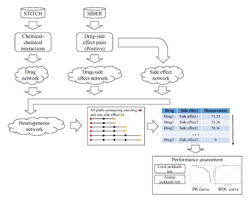
The study of drug side effects is a significant task in drug discovery. Candidate drugs with unaccepted side effects must be eliminated to prevent risks for both patients and pharmaceutical companies. Thus, all side effects for any candidate drug should be determined. However, this task, which is carried out through traditional experiments, is time-consuming and expensive. Building computational methods has been increasingly used for the identification of drug side effects. In the present study, a new path-based method was proposed to determine drug side effects. A heterogeneous network was built to perform such method, which defined drugs and side effects as nodes. For any drug and side effect, the proposed path-based method determined all paths with limited length that connects them and further evaluated the association between them based on these paths. The strong association indicates that the drug has a side effect with a high probability. By using two types of jackknife test, the method yielded good performance and was superior to some other network-based methods. Furthermore, the effects of one parameter in the method and heterogeneous network was analyzed.
Citation: Meng Jiang, Bo Zhou, Lei Chen. Identification of drug side effects with a path-based method[J]. Mathematical Biosciences and Engineering, 2022, 19(6): 5754-5771. doi: 10.3934/mbe.2022269
The study of drug side effects is a significant task in drug discovery. Candidate drugs with unaccepted side effects must be eliminated to prevent risks for both patients and pharmaceutical companies. Thus, all side effects for any candidate drug should be determined. However, this task, which is carried out through traditional experiments, is time-consuming and expensive. Building computational methods has been increasingly used for the identification of drug side effects. In the present study, a new path-based method was proposed to determine drug side effects. A heterogeneous network was built to perform such method, which defined drugs and side effects as nodes. For any drug and side effect, the proposed path-based method determined all paths with limited length that connects them and further evaluated the association between them based on these paths. The strong association indicates that the drug has a side effect with a high probability. By using two types of jackknife test, the method yielded good performance and was superior to some other network-based methods. Furthermore, the effects of one parameter in the method and heterogeneous network was analyzed.

| [1] |
S. Shabani-Mashcool, S. A. Marashi, S. Gharaghani, NDDSA: A network- and domain-based method for predicting drug-side effect associations, Inform. Process. Manag., 57 (2020), 102357. https://doi.org/10.1016/j.ipm.2020.102357 doi: 10.1016/j.ipm.2020.102357

|
| [2] |
Y. J. Ding, J. J. Tang, F. Guo, Identification of drug-side effect association via multiple information integration with centered kernel alignment, Neurocomputing, 325 (2019), 211–224. https://doi.org/10.1016/j.neucom.2018.10.028 doi: 10.1016/j.neucom.2018.10.028
|
| [3] |
A. Lakizadeh, S. M. H. Mir-Ashrafi, Drug repurposing improvement using a novel data integration framework based on the drug side effect, Inform. Med. Unlocked, 23 (2021), 100523. https://doi.org/10.1016/j.imu.2021.100523 doi: 10.1016/j.imu.2021.100523
|
| [4] |
E. Pauwels, V. Stoven, Y. Yamanishi, Predicting drug side-effect profiles: a chemical fragment-based approach, BMC Bioinformatics, 12 (2011), 169. https://doi.org/10.1186/1471-2105-12-169 doi: 10.1186/1471-2105-12-169
|
| [5] |
S. Jamal, S. Goyal, A. Shanker, A. Grover, Predicting neurological adverse drug reactions based on biological, chemical and phenotypic properties of drugs using machine learning models, Sci. Rep., 7 (2017), 872. https://doi.org/10.1038/s41598-017-00908-z doi: 10.1038/s41598-017-00908-z
|
| [6] |
Y. Zheng, H. Peng, S. Ghosh, C. Lan, J. Li, Inverse similarity and reliable negative samples for drug side-effect prediction, BMC Bioinformatics, 19 (2019), 554. https://doi.org/10.1186/s12859-018-2563-x doi: 10.1186/s12859-018-2563-x
|
| [7] |
M. Liu, Y. Wu, Y. Chen, J. Sun, Z. Zhao, X. W. Chen, et al., Large-scale prediction of adverse drug reactions using chemical, biological, and phenotypic properties of drugs, J. Am. Med. Inform. Assoc., 19 (2012), e28–35. https://doi.org/10.1136/amiajnl-2011-000699 doi: 10.1136/amiajnl-2011-000699
|
| [8] |
S. Dey, H. Luo, A. Fokoue, J. Hu, P. Zhang, Predicting adverse drug reactions through interpretable deep learning framework, BMC Bioinformatics, 19 (2018), 476. https://doi.org/10.1186/s12859-018-2544-0 doi: 10.1186/s12859-018-2544-0
|
| [9] |
L. Chen, T. Huang, J. Zhang, M. Y. Zheng, K. Y. Feng, Y. D. Cai, et al., Predicting drugs side effects based on chemical-chemical interactions and protein-chemical interactions, BioMed Res. Int., 2013 (2013), 485034. https://doi.org/10.1155/2013/485034 doi: 10.1155/2013/485034
|
| [10] |
W. Zhang, F. Liu, L. Luo, J. Zhang, Predicting drug side effects by multi-label learning and ensemble learning, BMC Bioinformatics, 16 (2015), 365. https://doi.org/10.1186/s12859-015-0774-y doi: 10.1186/s12859-015-0774-y
|
| [11] |
N. Atias, R. Sharan, An algorithmic framework for predicting side effects of drugs, J. Comput. Biol., 18 (2011), 207–218. https://doi.org/10.1089/cmb.2010.0255 doi: 10.1089/cmb.2010.0255
|
| [12] |
E. Muñoz, V. Novácek, P. Y. Vandenbussche, Facilitating prediction of adverse drug reactions by using knowledge graphs and multi-label learning models, Brief. Bioinform., 20 (2017), 190–202. https://doi.org/10.1093/bib/bbx099 doi: 10.1093/bib/bbx099
|
| [13] | W. Zhang, Y. Chen, S. Tu, F. Liu, Q. Qu, Drug side effect prediction through linear neighborhoods and multiple data source integration, in IEEE International Conference on Bioinformatics and Biomedicine, (2016), 427–434. https://doi.org/10.1109/BIBM.2016.7822555 |
| [14] | E. Munoz, V. Novacek, P. Y. Vandenbussche, Using drug similarities for discovery of possible adverse reactions, AMIA Annu. Symp. Proc., 2016 (2016), 924–933. |
| [15] |
X. Zhao, L. Chen, J. Lu, A similarity-based method for prediction of drug side effects with heterogeneous information, Math. Biosci., 306 (2018), 136–144. https://doi.org/10.1016/j.mbs.2018.09.010 doi: 10.1016/j.mbs.2018.09.010
|
| [16] |
H. Liang, L. Chen, X. Zhao, X. Zhang, Prediction of drug side effects with a refined negative sample selection strategy, Comput. Math. Method. M., 2020 (2020), 1573543. https://doi.org/10.1155/2020/1573543 doi: 10.1155/2020/1573543
|
| [17] |
X. Zhao, L. Chen, Z. H. Guo, T. Liu, Predicting drug side effects with compact integration of heterogeneous networks, Curr. Bioinform., 14 (2019), 709–720. https://doi.org/10.2174/1574893614666190220114644 doi: 10.2174/1574893614666190220114644
|
| [18] |
X. Guo, W. Zhou, Y. Yu, Y. Ding, J. Tang, F. Guo, A novel triple matrix factorization method for detecting drug-side effect association based on kernel target alignment, BioMed Res. Int., 2020 (2020), 4675395. https://doi.org/10.1155/2020/4675395 doi: 10.1155/2020/4675395
|
| [19] |
Y. Ding, J. Tang, F. Guo, Identification of drug-side effect association via semi-supervised model and multiple kernel learning, IEEE J. Biomed. Health, 23 (2019), 2619–2632. https://doi.org/10.1109/JBHI.2018.2883834 doi: 10.1109/JBHI.2018.2883834
|
| [20] | H. Tong, C. Faloutsos, J. Pan, Fast random walk with restart and its applications, in Sixth International Conference on Data Mining, (2006), 613–622. https://doi.org/10.1109/ICDM.2006.70 |
| [21] |
D. E. Carlin, B. Demchak, D. Pratt, E. Sage, T. Ideker, Network propagation in the cytoscape cyberinfrastructure, PLoS Comput. Biol., 13 (2017), e1005598. https://doi.org/10.1371/journal.pcbi.1005598 doi: 10.1371/journal.pcbi.1005598
|
| [22] |
M. Kuhn, M. Campillos, I. Letunic, L. J. Jensen, P. Bork, A side effect resource to capture phenotypic effects of drugs, Mol. Syst. Biol., 6 (2010), 343. https://doi.org/10.1038/msb.2009.98 doi: 10.1038/msb.2009.98
|
| [23] |
M. Kuhn, D. Szklarczyk, S. Pletscher-Frankild, T. H. Blicher, C. von Mering, L. J. Jensen, et al., STITCH 4: integration of protein–chemical interactions with user data, Nucleic Acids Res., 42 (2014), D401–D407. https://doi.org/10.1093/nar/gkt1207 doi: 10.1093/nar/gkt1207
|
| [24] |
D. Weininger, SMILES, a chemical language and information system. 1. Introduction to methodology and encoding rules, J. Chem. Inf. Comput. Sci., 28 (1988), 31–36. https://doi.org/10.1021/ci00057a005 doi: 10.1021/ci00057a005
|
| [25] |
X. Xiao, W. Zhu, B. Liao, J. Xu, C. Gu, B. Ji, et al., BPLLDA: predicting lncRNA-Disease associations based on simple paths with limited lengths in a heterogeneous network, Front. Genet., 9 (2018), 411. https://doi.org/10.3389/fgene.2018.00411 doi: 10.3389/fgene.2018.00411
|
| [26] |
W. Ba-Alawi, O. Soufan, M. Essack, P. Kalnis, V. B. Bajic, DASPfind: new efficient method to predict drug-target interactions, J. Cheminformatics, 8 (2016), 15. https://doi.org/10.1186/s13321-016-0128-4 doi: 10.1186/s13321-016-0128-4
|
| [27] |
Z. H. You, Z. A. Huang, Z. Zhu, G. Y. Yan, Z. W. Li, Z. Wen, et al., PBMDA: a novel and effective path-based computational model for miRNA-disease association prediction, PLoS Comput. Biol., 13 (2017), e1005455. https://doi.org/10.1371/journal.pcbi.1005455 doi: 10.1371/journal.pcbi.1005455
|
| [28] |
J. Gao, B. Hu, L. Chen, A path-based method for identification of protein phenotypic annotations, Curr. Bioinform., 16 (2021), 1214–1222. https://doi.org/10.2174/1574893616666210531100035 doi: 10.2174/1574893616666210531100035
|
| [29] |
S. Kohler, S. Bauer, D. Horn, P. N. Robinson, Walking the interactome for prioritization of candidate disease genes, Am. J. Hum. Genet., 82 (2008), 949–958. https://doi.org/10.1016/j.ajhg.2008.02.013 doi: 10.1016/j.ajhg.2008.02.013
|
| [30] |
Y.J. Li, J. C. Patra, Genome-wide inferring gene-phenotype relationship by walking on the heterogeneous network, Bioinformatics, 26 (2010), 1219–1224. https://doi.org/10.1093/bioinformatics/btq108 doi: 10.1093/bioinformatics/btq108
|
| [31] |
X. Chen, M. X. Liu, G. Y. Yan, Drug-target interaction prediction by random walk on the heterogeneous network, Mol. BioSyst., 8 (2012), 1970–1978. https://doi.org/10.1039/C2MB00002D doi: 10.1039/C2MB00002D
|
| [32] |
L. Chen, T. Liu, X. Zhao, Inferring anatomical therapeutic chemical (ATC) class of drugs using shortest path and random walk with restart algorithms, BBA Mol. Basis Dis., 1864 (2017), 2228–2240. https://doi.org/10.1016/j.bbadis.2017.12.019 doi: 10.1016/j.bbadis.2017.12.019
|
| [33] |
L. Chen, Y. H. Zhang, Z. Zhang, T. Huang, Y. D. Cai, Inferring novel tumor suppressor genes with a protein-protein interaction network and network diffusion algorithms, Mol. Ther. Methods Clin. Dev., 10 (2018), 57–67. https://doi.org/10.1016/j.omtm.2018.06.007 doi: 10.1016/j.omtm.2018.06.007
|
| [34] |
S. Lu, K. Zhao, X. Wang, H. Liu, X. Ainiwaer, Y. Xu, et al., Use of laplacian heat diffusion algorithm to infer novel genes with functions related to uveitis, Front. Genet., 9 (2018), 425. https://doi.org/10.3389/fgene.2018.00425 doi: 10.3389/fgene.2018.00425
|
| [35] |
H. Y. Liang, B. Hu, L. Chen, S. Q. Wang, Aorigele, Recognizing novel chemicals/drugs for anatomical therapeutic chemical classes with a heat diffusion algorithm, BBA Mol. Basis. Dis., 1866 (2020), 165910. https://doi.org/10.1016/j.bbadis.2020.165910 doi: 10.1016/j.bbadis.2020.165910
|
| [36] |
M. Imanishi, Y. Hori, M. Nagaoka, Y. Sugiura, Design of novel zinc finger proteins: towards artificial control of specific gene expression, Eur. J. Pharm. Sci., 13 (2001), 91–97. https://doi.org/10.1016/S0928-0987(00)00212-8 doi: 10.1016/S0928-0987(00)00212-8
|
| [37] |
M. Alirezaei, E. Mordelet, N. Rouach, A. C. Nairn, J. Glowinski, J. Premont, Zinc-induced inhibition of protein synthesis and reduction of connexin-43 expression and intercellular communication in mouse cortical astrocytes, Eur. J. Neurosci., 16 (2002), 1037–1044. https://doi.org/10.1046/j.1460-9568.2002.02180.x doi: 10.1046/j.1460-9568.2002.02180.x
|
| [38] |
K. H. Ibs, L. Rink, Zinc-altered immune function, J. Nutr., 133 (2003), 1452s–1456s. https://doi.org/10.1093/jn/133.5.1452S doi: 10.1093/jn/133.5.1452S
|
| [39] |
Z. A. Bhutta, R. E. Black, K. H. Brown, J. M. Gardner, S. Gore, A. Hidayat, et al., Prevention of diarrhea and pneumonia by zinc supplementation in children in developing countries: Pooled analysis of randomized controlled trials, J. Pediatr., 135 (1999), 689–697. https://doi.org/10.1016/S0022-3476(99)70086-7 doi: 10.1016/S0022-3476(99)70086-7
|
| [40] |
D. E. Roth, S. A. Richard, R. E. Black, Zinc supplementation for the prevention of acute lower respiratory infection in children in developing countries: meta-analysis and meta-regression of randomized trials, Int. J. Epidemiol., 39 (2010), 795–808. https://doi.org/10.1093/ije/dyp391 doi: 10.1093/ije/dyp391
|
| [41] |
D. Hulisz, Efficacy of zinc against common cold viruses: an overview, J. Am. Pharm. Assoc., 44 (2004), 594–603. https://doi.org/10.1331/1544-3191.44.5.594.Hulisz doi: 10.1331/1544-3191.44.5.594.Hulisz
|
| [42] |
R. O. Suara, J. E. Crowe, Effect of zinc salts on respiratory syncytial virus replication, Antimicrob. Agents Ch., 48 (2004), 783–790. https://doi.org/10.1128/AAC.48.3.783-790.2004 doi: 10.1128/AAC.48.3.783-790.2004
|
| [43] | D. Li, L. Z. Wen, H. Yuan, Observation on clinical efficacy of combined therapy of zinc supplement and jinye baidu granule in treating human cytomegalovirus infection, Zhongguo Zhong xi yi jie he za zhi, 25 (2005), 449–451. |
| [44] |
F. Femiano, F. Gombos, C. Scully, Recurrent herpes labialis: a pilot study of the efficacy of zinc therapy, J. Oral Pathol. Med., 34 (2005), 423–425. https://doi.org/10.1111/j.1600-0714.2005.00327.x doi: 10.1111/j.1600-0714.2005.00327.x
|
| [45] |
M. Singh, R. R. Das, Zinc for the common cold, Cochrane Database Syst. Rev., 6 (2013), CD001364. https://doi.org/10.1002/14651858.CD001364.pub4 doi: 10.1002/14651858.CD001364.pub4
|
| [46] |
M. Lazzerini, H. Wanzira, Oral zinc for treating diarrhoea in children, Cochrane Database Syst. Rev., 12 (2016), CD005436. https://doi.org/10.1002/14651858.CD005436.pub5 doi: 10.1002/14651858.CD005436.pub5
|
| [47] |
F. Sakai, S. Yoshida, S. Endo, H. Tomita, Double-blind, placebo-controlled trial of zinc picolinate for taste disorders, Acta oto-laryngol., 122 (2002), 129–133. https://doi.org/10.1080/00016480260046517 doi: 10.1080/00016480260046517
|
| [48] | A. R. Watson, A. Stuart, F. E. Wells, I. B. Houston, G. M. Addison, Zinc supplementation and its effect on taste acuity in children with chronic renal failure, Hum. Nutr. Clin. Nutr., 37 (1983), 219–225. |
| [49] |
J. Cervantes, A. E. Eber, M. Perper, V. M. Nascimento, K. Nouri, J. E. Keri, The role of zinc in the treatment of acne: A review of the literature, Dermatol. Ther., 31 (2018), e12576. https://doi.org/10.1111/dth.12576 doi: 10.1111/dth.12576
|
| [50] | A. Y. Bedikian, M. Valdivieso, L. K. Heilbrun, R. H. Withers, G. P. Bodey, E. J. Freireich, Glycerol: an alternative to dexamethasone for patients receiving brain irradiation for metastatic disease, South. Med. J., 73 (1980), 1210–1214. |
| [51] |
M. S. Frank, M. C. Nahata, M. D. Hilty, Glycerol: a review of its pharmacology, pharmacokinetics, adverse reactions, and clinical use, Pharmacotherapy, 1 (1981), 147–160. https://doi.org/10.1002/j.1875-9114.1981.tb03562.x doi: 10.1002/j.1875-9114.1981.tb03562.x
|
| [52] |
J. Wang, Y. Ren, S. F. Wang, L. D. Kan, L. J. Zhou, H. M. Fang, et al., Comparative efficacy and safety of glycerol versus mannitol in patients with cerebral oedema and elevated intracranial pressure: A systematic review and meta-analysis, J. Clin. Pharm. Ther., 46 (2021), 504–514. https://doi.org/10.1111/jcpt.13314 doi: 10.1111/jcpt.13314
|
| [53] |
J. Wang, Y. Ren, L. J. Zhou, L. D. Kan, H. Fan, H. M. Fang, Glycerol Infusion Versus Mannitol for Cerebral Edema: A Systematic Review and Meta-analysis, Clin. Ther., 43 (2021), 637–649. https://doi.org/10.1016/j.clinthera.2021.01.010 doi: 10.1016/j.clinthera.2021.01.010
|
| [54] |
E. Righetti, M. G. Celani, T. A. Cantisani, R. Sterzi, G. Boysen, S. Ricci, Glycerol for acute stroke, Cochrane Database Syst. Rev., 2 (2004), CD000096. https://doi.org/10.1002/14651858.CD000096.pub2 doi: 10.1002/14651858.CD000096.pub2
|
| [55] |
A. Frei, C. Cottier, P. Wunderlich, E. Lüdin, Glycerol and dextran combined in the therapy of acute stroke. A placebo-controlled, double-blind trial with a planned interim analysis, Stroke, 18 (1987), 373–379. https://doi.org/10.1161/01.STR.18.2.373 doi: 10.1161/01.STR.18.2.373
|
| [56] |
E. Lin, Glycerol utilization and its regulation in mammals, Annu. Rev. Biochem., 46 (1977), 765–795. https://doi.org/10.1146/annurev.bi.46.070177.004001 doi: 10.1146/annurev.bi.46.070177.004001
|
| [57] |
Y. Yu, C. Kumana, I. Lauder, Y. Cheung, F. Chan, M. Kou, et al., Treatment of acute cortical infarct with intravenous glycerol. A double-blind, placebo-controlled randomized trial, Stroke, 24 (1993), 1119–1124. https://doi.org/10.1161/01.STR.24.8.1119 doi: 10.1161/01.STR.24.8.1119
|
| [58] |
B. á Rogvi-Hansen, G. Boysen, Intravenous Glycerol Treatment of Acute Stroke – A Statistical Review, Cerebrovasc. Dis., 2 (1992), 11–13. https://doi.org/10.1159/000108981 doi: 10.1159/000108981
|
| [59] |
H. L. Philpott, S. Nandurkar, J. Lubel, P. R. Gibson, Drug-induced gastrointestinal disorders, Frontline Gastroente., 5 (2014), 49–57. http://dx.doi.org/10.1136/flgastro-2013-100316 doi: 10.1136/flgastro-2013-100316
|
| [60] | S. Saleem, How to induce arrhythmias with dopamine, in Arrhythmia Induction in the EP Lab, Springer, (2019), 81–89. https://doi.org/10.1007/978-3-319-92729-9_9 |
| [61] |
R. Ceravolo, C. Rossi, E. Del Prete, U. Bonuccelli, A review of adverse events linked to dopamine agonists in the treatment of Parkinson's disease, Expert Opin. Drug Saf., 15 (2016), 181–198. https://doi.org/10.1517/14740338.2016.1130128 doi: 10.1517/14740338.2016.1130128
|
 mbe-19-06-269-supplementary.pdf mbe-19-06-269-supplementary.pdf |
 |


Figures(6) / Tables(3)

Meng Jiang, Bo Zhou, Lei Chen. Identification of drug side effects with a path-based method[J]. Mathematical Biosciences and Engineering, 2022, 19(6): 5754-5771. doi: 10.3934/mbe.2022269


 DownLoad: