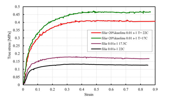
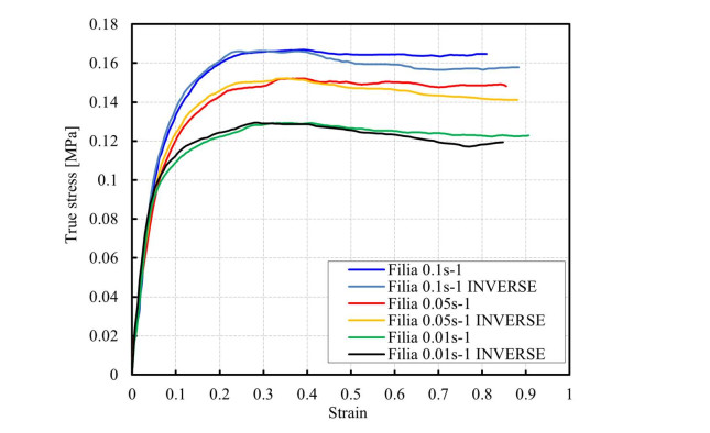
The article discusses the selected mechanical and plastic properties of modelling materials based on plasticine and filia wax utilized in the physical modelling. Application of the physical modelling with the utilize of soft model materials as well as plasticine and waxes with different inoculants, is a frequently used method applied as an alternative or verification of FE modelling of volumetric plastic working processes. First, in the ring test, the friction coefficients for the base model materials for various lubricants were determined. Then, in the compression test, the flow curves for model materials modified with various modifying substances (kaolin, lanolin, paraffin, chalk, etc.) were determined. The last step of the research studies was to verify the correctness of determining the flow curves using the inverse method. Based on the research carried out, a database was developed for soft model materials, covering the entire spectrum of flow curves and selected mechanical (friction coefficient, true and critical stress) and plastic properties (plastic deformation), which allows the selection of an appropriate mixture of model material to the real metallic material. Based on the obtained results, it can be concluded that both in the case of plasticine and filia wax, both of these materials together with modifiers very well simulate the behavior of warm and hot deformed metallic materials (with softening), much worse for materials with a clear hardening, characterizing cold work. In the case of filia wax, more stable properties were observed compared to plasticine-based materials.
Citation: Marek Hawryluk, Jan Marzec, Tatiana Karczewska, Łukasz Dudkiewicz. Determination of the characteristics and mechanical properties for soft materials based on plasticine and filia wax with inoculants[J]. AIMS Materials Science, 2022, 9(2): 325-343. doi: 10.3934/matersci.2022020
The article discusses the selected mechanical and plastic properties of modelling materials based on plasticine and filia wax utilized in the physical modelling. Application of the physical modelling with the utilize of soft model materials as well as plasticine and waxes with different inoculants, is a frequently used method applied as an alternative or verification of FE modelling of volumetric plastic working processes. First, in the ring test, the friction coefficients for the base model materials for various lubricants were determined. Then, in the compression test, the flow curves for model materials modified with various modifying substances (kaolin, lanolin, paraffin, chalk, etc.) were determined. The last step of the research studies was to verify the correctness of determining the flow curves using the inverse method. Based on the research carried out, a database was developed for soft model materials, covering the entire spectrum of flow curves and selected mechanical (friction coefficient, true and critical stress) and plastic properties (plastic deformation), which allows the selection of an appropriate mixture of model material to the real metallic material. Based on the obtained results, it can be concluded that both in the case of plasticine and filia wax, both of these materials together with modifiers very well simulate the behavior of warm and hot deformed metallic materials (with softening), much worse for materials with a clear hardening, characterizing cold work. In the case of filia wax, more stable properties were observed compared to plasticine-based materials.

| [1] |
Hawryluk M, Polak S, Gronostajski Z, et al. (2019) Application of physical similarity utilizing soft modeling materials and numerical simulations to analyses the plastic flow of uc1 steel and the evolution of forces in a specific multi-operational industrial precision forging process with a constant-velocity joint housing. Exp Tech 43: 225-235. https://doi.org/10.1007/s40799-018-0288-4 doi: 10.1007/s40799-018-0288-4

|
| [2] |
Vazquez V, Altan T (2000) New concepts in die design—physical and computer modeling applications. J Mater Process Technol 98: 212-223. https://doi.org/10.1016/S0924-0136(99)00202-2 doi: 10.1016/S0924-0136(99)00202-2
|
| [3] |
Arentoft M, Gronostajski Z, Niechajowicz A, et al. (2000) Physical and mathematical modelling of extrusion processes. J Mater Process Technol 106: 2-7. https://doi.org/10.1016/S0924-0136(00)00629-4 doi: 10.1016/S0924-0136(00)00629-4
|
| [4] |
Lee RS, Blazynski TZ (1984) Mechanical properties of a composite wax model material simulating plastic flow of metals. J Mech Work Technol 9: 301-312. https://doi.org/10.1016/0378-3804(84)90111-6 doi: 10.1016/0378-3804(84)90111-6
|
| [5] | Oudin J, Ravalard Y, Rommens S (1980) On the contribution of waxes to the simulation of metal forming processes, North American Manufacturing Research Conference Proceedings, Rolla: University of Missouri-Rolla, 166-170. |
| [6] |
Finér S, Kivivuori S, Kleemola H (1985) Stress—Strain relationships of wax-based model materials. J Mech Work Technol 12: 269-277. https://doi.org/10.1016/0378-3804(85)90142-1 doi: 10.1016/0378-3804(85)90142-1
|
| [7] |
Altan T, Henning HJ, Sabroff AM (1970) The use of model materials in predicting forming loads in metalworking. ASME J Eng Ind 92: 444-451. https://doi.org/10.1115/1.3427776 doi: 10.1115/1.3427776
|
| [8] | Finer S, Kivivuori S, Kleemola H (1982) Mekaniska och termiska egenskaper av modellmaterial. Del 1: Modellvaxet Filia: SIMON-rapport, Espoo: VTT Technical Research Centre of Finland. |
| [9] |
Farzad A, Blazynski TZ (1989) Geometry factor and redundancy effects in extrusion of rod. J Mech Work Technol 19: 357-372. https://doi.org/10.1016/0378-3804(89)90082-X doi: 10.1016/0378-3804(89)90082-X
|
| [10] |
Eckerson K, Liechty B, Sorensen CD (2008) Thermomechanical similarity between Van Aken plasticine and metals in hot-forming processes. J Strain Anal Eng Des 43: 383-394. https://doi.org/10.1243/03093247JSA364 doi: 10.1243/03093247JSA364
|
| [11] |
Sharma M, Singh AK, Singh P, et al. (2011) Experimental investigation of the effect of die angle on extrusion process using plasticine. Exp Tech 35: 38-44. https://doi.org/10.1111/j.1747-1567.2010.00655.x doi: 10.1111/j.1747-1567.2010.00655.x
|
| [12] |
Azushima A, Kudo H (1987) Physical simulation for metal forming with strain rate sensitive model material. Adv Tech Plast 2: 1221-1227. https://doi.org/10.1007/978-3-662-11046-1_68 doi: 10.1007/978-3-662-11046-1_68
|
| [13] |
Schö pfer MPJ, Zulauf G (2002) Strain-dependent rheology and the memory of plasticine. Tectonophysics 354: 85-99. https://doi.org/10.1016/S0040-1951(02)00292-5 doi: 10.1016/S0040-1951(02)00292-5
|
| [14] | Arentoft M (1997) Prevention of Defects in Forging by Numerical and Physical Simulation, Copenhagen: Technical University of Denmark. |
| [15] |
Gouveia BPPA, Rodrigues JMC, Martins PAF, et al. (2001) Physical modelling and numerical simulation of the round-to-square forward extrusion. J Mater Process Tech 112: 244-251. https://doi.org/10.1016/S0924-0136(01)00725-7 doi: 10.1016/S0924-0136(01)00725-7
|
| [16] | Gingher GC, Padjen G (1993) Hot strip mill edging practices and plasticine modelling, 34 th Mechanical Working and Steel Processing Conference Proceedings, Montreal: Iron and Steel Society of AIME, 3-12. |
| [17] | Hawryluk M (2006) The influence of the condition of plastic similarity on the accuracy of physical modeling of extrusion processes[Dissertation]. Wroclaw University of Science and Technology (in Polish). Available from: http://www.itshc.pwr.edu.pl/language/en/dissertation. |
| [18] |
Boucly P, Oudin J, Ravalard Y (1988) Simulation of ring rolling with new wax-based model materials on a flexible experimental machine. J Mech Work Technol 16: 119-143. https://doi.org/10.1016/0378-3804(88)90156-8 doi: 10.1016/0378-3804(88)90156-8
|
| [19] |
Adams MJ (1989) A two roll mill as a rheometer for pastes, material resume social symposium process. Mater Res Soc 289: 237-257. https://doi.org/10.1557/PROC-289-245 doi: 10.1557/PROC-289-245
|
| [20] |
Shin HW, Kim DW, Kim N (1994) A study of the rolling of I-section beams. Int J Mach Tools Manuf 34: 147-160. https://doi.org/10.1016/0890-6955(94)90097-3 doi: 10.1016/0890-6955(94)90097-3
|
| [21] |
Moon YH, Chun MS, Yi JJ, et al. (1993) Physical modelling of edge rolling in plate mill with plasticine. Steel Res 64: 557-563. https://doi.org/10.1002/srin.199301571 doi: 10.1002/srin.199301571
|
| [22] |
Mohammadi MM, Sadeghi MH (2010) Simulation and physical modeling of forging sequence of Bj type outer race. Adv Mater Res 83: 150-156. https://doi.org/10.4028/www.scientific.net/AMR.83-86.150 doi: 10.4028/www.scientific.net/AMR.83-86.150
|
| [23] |
Pertence AEM, Cetlin PR (2000) Similarity of ductility between model and real materials. J Mater Process Technol 103: 434-438. https://doi.org/10.1016/S0924-0136(00)00513-6 doi: 10.1016/S0924-0136(00)00513-6
|
| [24] |
Danckert J, Wanheim T (1976) Slipline wax: An easy way to determine the slipline field in specimens subjected to plastic deformation under plane-strain conditions. Exp Mech 16: 318-320. https://doi.org/10.1007/BF02324022 doi: 10.1007/BF02324022
|
| [25] | Gronostajski Z, Hawryluk M, Zwierzchowski M, et al. (2008) Analysis of forging process of constatnt velocity joint body. Steel Res Int 1: 547-554. |
| [26] |
Wójcik Ł, Lis K, Pater Z (2016) Plastometric tests for plasticine as physical modelling material. Open Eng 6: 653-659. https://doi.org/10.1515/eng-2016-0093 doi: 10.1515/eng-2016-0093
|
| [27] | Alder J, Phillips KA (1954) The effect of strain-rate and temperature on the resistance of aluminum, copper and steel to compression. J Inst Met 83: 80-86. |
| [28] |
Sofuoglu H, Rasty J (1999) On the measurement of friction coefficient utilizing the ring compression test. Tribol Int 32: 327-335. https://doi.org/10.1016/S0301-679X(99)00055-9 doi: 10.1016/S0301-679X(99)00055-9
|
| [29] |
Petersen SB, Martins PAF, Bay N (1998) An alternative ring-test geometry for the evaluation of friction under low normal pressure. J Mater Process Technol 79: 14-24. https://doi.org/10.1016/S0924-0136(97)00448-2 doi: 10.1016/S0924-0136(97)00448-2
|
| [30] |
Bay N, Lassen S, Pedersen CD, et al. (1991) Lubrication limits in backward can extrusion at low reductions. CIRP Ann Manuf Technol 40: 239-242. https://doi.org/10.1016/S0007-8506(07)61977-5 doi: 10.1016/S0007-8506(07)61977-5
|
| [31] |
Bennani B, Bay N (1996) Limits of lubrication in backward can extrusion: analysis by the finite-element method and physical modelling experiments. J Mater Process Technol 61: 275-286. https://doi.org/10.1016/0924-0136(95)02181-7 doi: 10.1016/0924-0136(95)02181-7
|
| [32] |
Shen G, Vedhanayagram A, Kropp E, et al. (1992) A method for evaluating friction using a backward extrusion-type forging. J Mech Work Technol 33: 109-123. https://doi.org/10.1016/0924-0136(92)90314-I doi: 10.1016/0924-0136(92)90314-I
|
| [33] | Hawryluk M, Wilk-Kołodziejczyk D, Regulski K, et al. (2019) Development of an approximation model of selected properties of model materials used for simulations of bulk metal plastic forming processes using induction of decision trees. Arch Metall Mater 64: 1073-1085. |
| [34] |
Gronostajski Z, Hawryluk M (2007) Analysis of metal forming processes by using physical modeling and new plastic similarity condition. AIP Conference Proceedings 9: 608-613. https://doi.org/10.1063/1.2729580 doi: 10.1063/1.2729580
|
| [35] | Pietrzyk M, Lenard JG (1990) Finite element simulation during metal forming processes, International Heat Transfer Conference 9, Jerusalem: Begell House, 413-418. https: //doi.org/10.1615/IHTC9.1560 |
| [36] | Szeliga D, Pietrzyk M (2002) Identification of rheological and tribological parameters, Metal Forming Science and Practice, Amsterdam: Elsevier, 227-258. https: //doi.org/10.1016/B978-008044024-8/50012-6 |
| [37] |
Maropoulos PG (1995) Review of research in tooling technology, process modelling and process planning part Ⅱ: Process planning. Comput Integr Manuf Syst 8: 13-20. https://doi.org/10.1016/0951-5240(95)92809-9 doi: 10.1016/0951-5240(95)92809-9
|
| [38] | Chen CC, Kobayashi S (1979) Rigid-Plastic Finite-Element Analysis of Plastic Deformation in Metal-Forming Processes, Berkley: University of California. |
Figures(10) / Tables(4)

Marek Hawryluk, Jan Marzec, Tatiana Karczewska, Łukasz Dudkiewicz. Determination of the characteristics and mechanical properties for soft materials based on plasticine and filia wax with inoculants[J]. AIMS Materials Science, 2022, 9(2): 325-343. doi: 10.3934/matersci.2022020


 DownLoad: