Correlation structure networks of stock market during terrorism: evidence from Pakistan

Bilal Ahmed Memon; Hongxing Yao; Bilal Ahmed Memon; Hongxing Yao

doi:10.3934/DSFE.2021007

Data Science in Finance and Economics

2021, Volume 1, Issue 2: 117-140. doi: 10.3934/DSFE.2021007

Previous Article Next Article

Research article

Correlation structure networks of stock market during terrorism: evidence from Pakistan

Bilal Ahmed Memon ^{1
,
,},
Hongxing Yao ²

1.
Department of Business Administration, Iqra University, Karachi, Pakistan
2.
School of finance and economics, Jiangsu University, Zhenjiang, China

Received: 08 June 2021 Accepted: 13 July 2021 Published: 16 July 2021
JEL Codes: G10, B4, D53, D85, F36

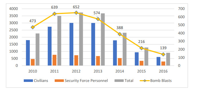
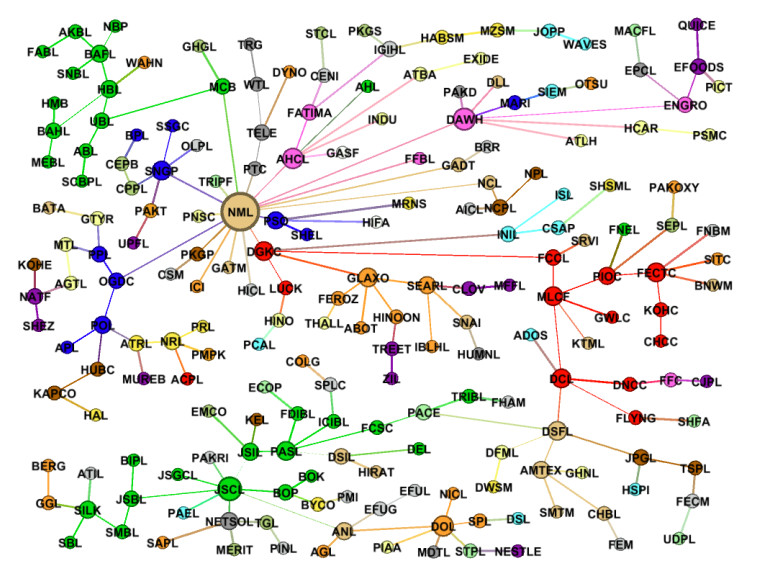
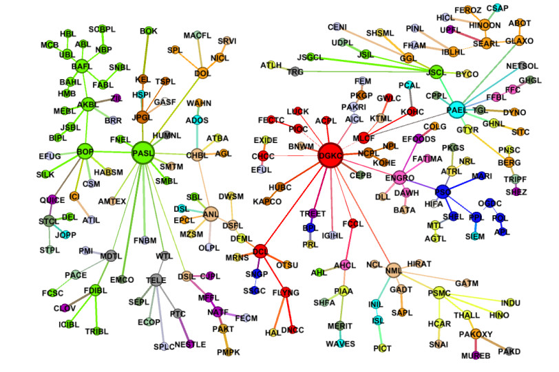
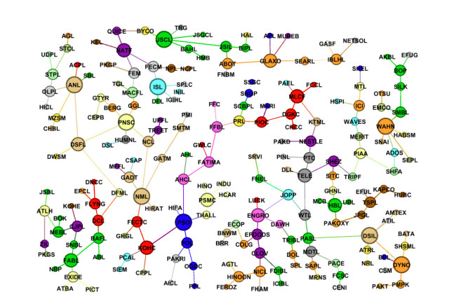
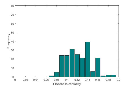
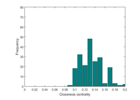
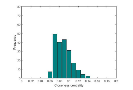
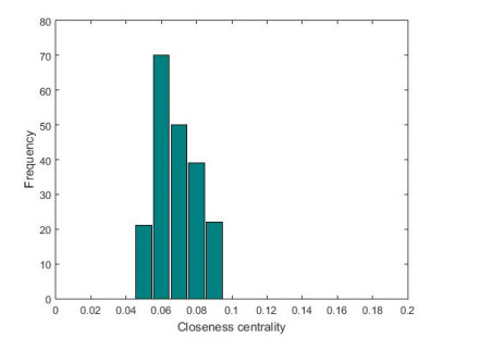
We study topology of correlation structures and construct Pearson correlation-based networks (MST-Pearson) and partial correlation-based networks (MST-Partial) during two time periods of extreme terrorist activities (High civilian and security forces fatalities) and relaxed period (low civilian and security forces fatalities). Our results find that probability density function of Pearson correlation coefficients for relaxed period and partial correlation coefficients for both periods slightly deviates from the gaussian function. MST-Pearson during the period of extreme terrorist activities is a crisis like less stable market structure in comparison with the meta-stable market state structure of relaxed period. Our studies also find presence of two most prominent clusters belonging to cement, and chemical and pharmaceutical sectors among four MSTs. In addition, we find important role of few sectors during the period of extreme terrorist activities in comparison with a more diversified sectoral role in the relaxed period. Furthermore, time varying topological properties indicate an expansion in both MST-Pearson and MST-Partial length in the relaxed period due to counter terrorism strategies. Thus, the study reveals interesting findings and implications for the policymakers and investors of Pakistan stock market during the event of terrorism.

Keywords:

Citation: Bilal Ahmed Memon, Hongxing Yao. Correlation structure networks of stock market during terrorism: evidence from Pakistan[J]. Data Science in Finance and Economics, 2021, 1(2): 117-140. doi: 10.3934/DSFE.2021007

Related Papers:

[1]	M. Mossa Al-Sawalha, Rasool Shah, Adnan Khan, Osama Y. Ababneh, Thongchai Botmart . Fractional view analysis of Kersten-Krasil'shchik coupled KdV-mKdV systems with non-singular kernel derivatives. AIMS Mathematics, 2022, 7(10): 18334-18359. doi: 10.3934/math.20221010
[2]	Ihsan Ullah, Aman Ullah, Shabir Ahmad, Hijaz Ahmad, Taher A. Nofal . A survey of KdV-CDG equations via nonsingular fractional operators. AIMS Mathematics, 2023, 8(8): 18964-18981. doi: 10.3934/math.2023966
[3]	Saima Rashid, Rehana Ashraf, Fahd Jarad . Strong interaction of Jafari decomposition method with nonlinear fractional-order partial differential equations arising in plasma via the singular and nonsingular kernels. AIMS Mathematics, 2022, 7(5): 7936-7963. doi: 10.3934/math.2022444
[4]	Aslı Alkan, Halil Anaç . The novel numerical solutions for time-fractional Fornberg-Whitham equation by using fractional natural transform decomposition method. AIMS Mathematics, 2024, 9(9): 25333-25359. doi: 10.3934/math.20241237
[5]	Rasool Shah, Abd-Allah Hyder, Naveed Iqbal, Thongchai Botmart . Fractional view evaluation system of Schrödinger-KdV equation by a comparative analysis. AIMS Mathematics, 2022, 7(11): 19846-19864. doi: 10.3934/math.20221087
[6]	Khalid Khan, Amir Ali, Manuel De la Sen, Muhammad Irfan . Localized modes in time-fractional modified coupled Korteweg-de Vries equation with singular and non-singular kernels. AIMS Mathematics, 2022, 7(2): 1580-1602. doi: 10.3934/math.2022092
[7]	Saima Rashid, Sobia Sultana, Bushra Kanwal, Fahd Jarad, Aasma Khalid . Fuzzy fractional estimates of Swift-Hohenberg model obtained using the Atangana-Baleanu fractional derivative operator. AIMS Mathematics, 2022, 7(9): 16067-16101. doi: 10.3934/math.2022880
[8]	Muammer Ayata, Ozan Özkan . A new application of conformable Laplace decomposition method for fractional Newell-Whitehead-Segel equation. AIMS Mathematics, 2020, 5(6): 7402-7412. doi: 10.3934/math.2020474
[9]	Khalid Khan, Amir Ali, Muhammad Irfan, Zareen A. Khan . Solitary wave solutions in time-fractional Korteweg-de Vries equations with power law kernel. AIMS Mathematics, 2023, 8(1): 792-814. doi: 10.3934/math.2023039
[10]	Musawa Yahya Almusawa, Hassan Almusawa . Numerical analysis of the fractional nonlinear waves of fifth-order KdV and Kawahara equations under Caputo operator. AIMS Mathematics, 2024, 9(11): 31898-31925. doi: 10.3934/math.20241533

Abstract

1. Introduction

Fractional order Kersten-Krasil'shchik (KK) coupled Korteweg-de Vries (KdV)-modified KdV (mKdV) systems have served as the focus of extensive research in recent years due to their potential use in a variety of disciplines, including fluid dynamics, nonlinear optics and plasma physics ^[1,2,3,4]. These systems are characterized by the presence of fractional derivatives, which introduce non-local and memory effects into the dynamics of the system ^[5,6,7,8]. The KK coupled KdV-mKdV system is a system of two coupled nonlinear partial differential equations, which describe the evolution of two waves in a dispersive medium. The first equation is the well-known KdV equation, which describes the propagation of small amplitude, long wavelength waves. The second equation is the mKdV equation, which describes the propagation of larger amplitude, shorter wavelength waves. The KK coupling term, which is a nonlinear and non-local term, describes the interaction between the two waves ^[3,4,7]. Li et al. delved into an epidemic model's analysis and comparisons with other mechanisms in 2018 ^[12], while Jin and Wang explored chemotaxis phenomena in 2016 ^[13]. He et al. focused on fixed-point and variational inequality problems for Hadamard manifolds in 2022 ^[14]; this was followed by He et al. discussing nonexpansive mapping algorithms in 2023 ^[15]. Chen et al. contributed to particle physics, discovering hidden-charm pentaquarks in 2021 ^[16]. Lyu et al. analyzed cavity dynamics in water entries ^[17], whereas Yang and Kai delved into nonlinear Schr $\ddot{o}$ dinger equations in 2023.

Time fractional Kersten-Krasil'shchik coupled KdV-mKdV nonlinear system and homogeneous two component time fractional coupled third order KdV systems are very important fractional nonlinear systems for describing the behaviour of waves in multi-component plasma and elaborate various nonlinear phenomena in plasma physics. Other studies have focused on the stability, existence and uniqueness of solutions for KK coupled KdV-mKdV systems of fractional order. In addition to these studies, there have been many other works that have explored the properties of fractional order KK coupled KdV-mKdV systems, such as their integrability, conservation laws and soliton interactions. Overall, the literature on fractional order KK coupled KdV-mKdV systems is rich and diverse, and it continues to grow as researchers explore new properties and applications of these systems ^[18,19,20].

There are several methods that have been proposed to solve the fractional KdV (fKdV) equation and the mKdV equation. One of these methods is the homotopy perturbation method; this method uses a perturbation series and a homotopy approach to solve nonlinear differential equations. It has been used to find approximate solutions to the fKdV equation ^[21]. The variational iteration method uses a variation of a trial solution to find approximate solutions to nonlinear differential equations. The homotopy analysis method uses a homotopy approach and a perturbation series to solve nonlinear differential equations. It has been used to find approximate solutions to the fKdV equation ^[22] and the mKdV equation ^[23]. The Adomian decomposition method uses a decomposition of the nonlinear term of a differential equation into a series of simpler functions. It has been used to find approximate solutions to the fKdV equation and the mKdV equation ^[24,25]. Yang and Kai, dynamical properties, modulation instability analysis and chaotic behaviors to the nonlinear coupled Schrodinger equation in fiber Bragg gratings ^[26]. Chen et al. presented a linear free energy relationship in chemistry in 2020 ^[27]. Luo et al. proposed a new gradient method for force identification in vehicle-bridge systems in 2022 ^[28]. Additionally, Chen et al. focused on adaptive control of underwater vehicles in 2022 ^[29]. Lastly, Gu, Li and Liao developed an evolutionary multitasking approach for solving nonlinear equation systems in 2024 ^[30]. These studies collectively offer significant insights and advancements across a broad spectrum of scientific research areas, enriching our understanding and methodologies in their respective domains.

The ADM is a powerful technique for solving nonlinear differential equations. Developed by George Adomian in the late 1980s, the ADM is based on the idea of decomposing the solution of a nonlinear equation into a series of simpler functions, known as Adomian polynomials. These polynomials are obtained by iteratively applying the nonlinear operator to a constant function ^[31,32]. The ADM has been applied to a wide range of nonlinear problems, including partial differential equations, integral equations and stochastic differential equations. One of the key advantages of the ADM is its ability to handle equations with singularities, such as those that arise in physics and engineering. In recent years, researchers have been exploring the use of the ADM in combination with other techniques, such as the ZZ transform. The ZZ transform is a mathematical tool that can be used to transform a nonlinear equation into a linear equation, making it easier to solve. By combining the ADM with the ZZ transform, researchers have been able to solve a wide range of nonlinear problems with greater efficiency and accuracy. Many researchers have used the ADM together with the ZZ transform to solve, for example, the nonlinear fractional partial differential equations in fluid dynamics, nonlinear integral equations in quantum mechanics and nonlinear fractional stochastic differential equations in finance. Overall, the ADM with the ZZ transform has been shown to be an efficient and flexible strategy for addressing nonlinear problems, with numerous potential applications in various fields ^[33,34].

The current work is organized as follows. In Section 2, some fundamental definitions of fractional calculus are provided. The basic ideas of the Aboodh transform and the ADM are described in Section 3. In Section 4, we build approximate solutions to fractional Kersten-Krasil'shchik coupled KdV-mKdV systems of partial differential equations. Section 5 contains the conclusions.

2. Preliminaries

Definition 2.1. For functions, the Aboodh transformation is achieved as follow:

$B = \left\{{U}({\varrho}): \exists M, {{n_1}}, {{n_2}} > 0,|{U}({\varrho})| < M e^{-{\varepsilon} {\varrho}}\right\},$

which is described as follows ^[33,34]:

$A\{{U}({\varrho})\} = \frac{1}{{\varepsilon}} \int_{0}^{\infty} {U}({\varrho}) e^{-{\varepsilon} {\varrho}} d {\varrho},\ \ {\varrho} > 0 \text { and } {{n_1}} \leq {\varepsilon} \leq {{n_2}}.$

Theorem 2.2. Consider $G$ and $F$ as the Aboodh and Laplace transformations, respectively, of $\textit U(\varrho)$ over the set $B$ ^[35,36]. Then

$\begin{equation} G({\varepsilon}) = \frac{F({\varepsilon})}{{\varepsilon}} . \end{equation}$

(2.1)

Generalizing the Laplace and Aboodh integral transformations, Zain Ul Abadin Zafar created the ZZ transformation ^[37]. The ZZ transform is described as follows.

Definition 2.3. For all values of $\varrho \geq 0$ , the Z-transform for the function $\textit U(\varrho)$ is $Z(\kappa, \varepsilon)$ , which can be expressed as follows ^[37]:

$Z Z({U}(\varrho)) = Z({\kappa}, {\varepsilon}) = {\varepsilon} \int_{0}^{\infty} {U}({\kappa} \varrho) e^{-{\varepsilon} \varrho} d \varrho.$

The Z-transform is linear in nature, just as the Laplace and Aboodh transforms. On the other hand, the Mittag-Leffler function (MLF) is an expansion of the exponential function:

$E_{{\delta}}(z) = \sum\limits_{m = 0}^{\infty} \frac{z^{m}}{\Gamma(1+m {\delta})}, \quad \operatorname{Re}({\delta}) > 0 .$

Definition 2.4. The Atangana-Baleanu-Caputo (ABC) derivative of a function ${U}(\varphi, \varrho)$ in the space $H^{1}(a, b)$ for ${{\beta}} \in \; (0, 1)$ has the following definition ^[38]:

${A B C}_{a} D_{\varrho}^{{{\beta}}} {U}(\varphi, \varrho) = \frac{{B}({{\beta}})}{-{{\beta}}+1} \int_{a}^{\varrho} {U}^{\prime}(\varphi, \varrho) E_{{{\beta}}}\left(\frac{-{{\beta}}(\varrho-\eta)^{{{\beta}}}}{-{{\beta}}+1}\right) d \eta .$

Definition 2.5. The Atangana-Baleanu Riemann-Liouville (ABR) derivative is a part of the space $H^{1}(a, b)$ . The derivative can be represented for any value of ${{\beta}} \in (0, 1)$ as follows ^[38]:

${ }_{a}^{A B R} D_{\varrho}^{{{\beta}}} {U}(\varphi, \eta) = \frac{{B}({{\beta}})}{-{{\beta}}+1} \frac{d}{d \varrho} \int_{a}^{\varrho} {U}(\varphi, \eta) E_{{{\beta}}}\left(\frac{-{{\beta}}(\varrho-\eta)^{{{\beta}}}}{-{{\beta}}+1}\right) d \eta.$

The property of the function ${B}({{\beta}})$ is that it tends to 1 for both 0 and 1. Additionally, $\forall \; {{\beta}} > 0$ , ${B}({{\beta}}) > {a}$ .

Theorem 2.6. The Laplace transformation for the ABR derivative and ABC derivative are given by ^[38]:

$\begin{equation} \mathrm{L}\left\{{ }_{a}^{A B C} D_{{\varrho}}^{{{\beta}}} {U}(\varphi, {\varrho})\right\}({\varepsilon}) = \frac{{B}({{\beta}})}{-{{\beta}}+1} \frac{{\varepsilon}^{{{\beta}}} L\{{U}(\varphi, {\varrho})\}-{\varepsilon}^{{{\beta}}-1} {U}(\varphi, 0)}{{\varepsilon}^{{{\beta}}}+\frac{{{\beta}}}{-{{\beta}}+1}} \end{equation}$

(2.2)

and

$\begin{equation} L\left\{\begin{array}{l} A B R \\ a \end{array} D_{{\varrho}}^{{{\beta}}} {U}(\varphi, {\varrho})\right\}({\varepsilon}) = \frac{{B}({{\beta}})}{-{{\beta}}+1} \frac{{\varepsilon}^{{{\beta}}} L\{{U}(\varphi, {\varrho})\}}{{\varepsilon}^{{{\beta}}}+\frac{{{\beta}}}{-{{\beta}}+1}}. \end{equation}$

(2.3)

In the theorems below we assume that ${U}({\varrho}) \in H^{1}(a, b)$ , where $b > a$ and ${{\beta}} \in (0, 1)$ .

Theorem 2.7. The Aboodh transform gives rise to a new ABR derivative, which is known as the Aboodh transformed ABR derivative ^[36]

$\begin{equation} G({\varepsilon}) = A\left\{\begin{array}{l} A B R \\ a \end{array} D_{{\varrho}}^{{{\beta}}} {U}(\varphi, {\varrho})\right\}({\varepsilon}) = \frac{1}{{\varepsilon}}\left[\frac{{B}({{\beta}})}{-{{\beta}}+1} \frac{{\varepsilon}^{{{\beta}}} L\{{U}(\varphi, {\varrho})\}}{{\varepsilon}^{{{\beta}}}+\frac{{{\beta}}}{-{{\beta}}+1}}\right]. \end{equation}$

(2.4)

Theorem 2.8. The Aboodh transformation of ABC derivative is defined as follows ^[36]:

$\begin{equation} \begin{split} G({\varepsilon}) = & A\left\{\begin{array}{l} A B C \\ a \end{array} D_{{\varrho}}^{{{\beta}}} {U}(\varphi, {\varrho})\right\}({\varepsilon}) = \frac{1}{{\varepsilon}}\left[\frac{{B}({{\beta}})}{-{{\beta}}+1} \frac{{\varepsilon}^{{{\beta}}} L\{{U}(\varphi, {\varrho})\}-{\varepsilon}^{{{\beta}}-1} {U}(\varphi, 0)}{{\varepsilon}^{{{\beta}}}+\frac{{{\beta}}}{-{{\beta}}+1}}\right]. \end{split} \end{equation}$

(2.5)

Theorem 2.9. The $\mathrm{ZZ}$ transformation of ${U}({\varrho}) = {\varrho}^{{{\beta}}-1}$ is defined as

$\begin{equation} Z({\kappa}, {\varepsilon}) = \Gamma({{\beta}})\left(\frac{{\kappa}}{{\varepsilon}}\right)^{{{\beta}}-1}. \end{equation}$

(2.6)

Proof. The Aboodh transformation of ${U}({\varrho}) = {\varrho}^{{{\beta}}}, \ \ {{\beta}} \geq 0$ is given by

$G({\varepsilon}) = \frac{\Gamma({{\beta}})}{{\varepsilon}^{{{\beta}}+1}}.$

$\text { Now, } \quad G\left(\frac{{\varepsilon}}{{\kappa}}\right) = \frac{\Gamma({{\beta}}) {\kappa}^{{{\beta}}+1}}{{\varepsilon}^{{{\beta}}+1}} \text {. }$

Applying Eq (2.6), we obtain

$Z({\kappa}, {\varepsilon}) = \frac{{\varepsilon}^{2}}{{\kappa}^{2}} G\left(\frac{{\varepsilon}}{{\kappa}}\right) = \frac{{\varepsilon}^{2}}{{\kappa}^{2}} \frac{\Gamma({{\beta}}) {\kappa}^{{{\beta}}+1}}{{\varepsilon}^{{{\beta}}+1}} = \Gamma({{\beta}})\left(\frac{{\kappa}}{{\varepsilon}}\right)^{{{\beta}}-1}.$

□

Theorem 2.10. Let ${{\beta}}$ and $\omega$ be complex numbers and assume that the real part of ${{\beta}}$ is greater than 0. The $\mathrm{ZZ}$ transformation of $E_{{{\beta}}}\left(\omega {\varrho}^{{{\beta}}}\right)$ can be defined as follows ^[36]:

$\begin{equation} Z Z\left\{\left(E_{{{\beta}}}\left(\omega {\varrho}^{{{\beta}}}\right)\right)\right\} = Z({\kappa}, {\varepsilon}) = \left(1-\omega\left(\frac{{\kappa}}{{\varepsilon}}\right)^{{{\beta}}}\right)^{-1}. \end{equation}$

(2.7)

Proof. The Aboodh transformation of $E_{{{\beta}}}\left(\omega {\varrho}^{{{\beta}}}\right)$ is defined as follows:

$\begin{equation} G({\varepsilon}) = \frac{F({\varepsilon})}{{\varepsilon}} = \frac{{\varepsilon}^{{{\beta}}-1}}{{\varepsilon}\left({\varepsilon}^{{{\beta}}}-\omega\right)}. \end{equation}$

(2.8)

So,

$\begin{equation} G\left(\frac{{\varepsilon}}{{\kappa}}\right) = \frac{\left(\frac{{\varepsilon}}{{\kappa}}\right)^{{{\beta}}-1}}{\left(\frac{{\varepsilon}}{{\kappa}}\right)\left(\left(\frac{{\varepsilon}}{{\kappa}}\right)^{{{\beta}}}-\omega\right)} \text {; } \end{equation}$

(2.9)

we obtain

$\begin{gathered} Z({\kappa}, {\varepsilon}) = \left(\frac{{\varepsilon}}{{\kappa}}\right)^{2} G\left(\frac{{\varepsilon}}{{\kappa}}\right) = \left(\frac{{\varepsilon}}{{\kappa}}\right)^{2} \frac{\left(\frac{{\varepsilon}}{{\kappa}}\right)^{{{\beta}}-1}}{\left(\frac{{\varepsilon}}{{\kappa}}\right)\left(\left(\frac{{\varepsilon}}{{\kappa}}\right)^{{{\beta}}}-\omega\right)} \\ = \frac{\left(\frac{{\varepsilon}}{{\kappa}}\right)^{{{\beta}}}}{\left(\frac{{\varepsilon}}{{\kappa}}\right)^{{{\beta}}}-\omega} = \left(1-\omega\left(\frac{{\kappa}}{{\varepsilon}}\right)^{{{\beta}}}\right)^{-1}. \end{gathered}$

□

Theorem 2.11. The ZZ transform of the ABC derivative can be defined as follows: If $G({\varepsilon})$ and $Z({\kappa}, {\varepsilon})$ are the ZZ and Aboodh transformations of ${U}({\varrho})$ , respectively ^[36], they we have

$\begin{equation} Z Z\left\{\begin{array}{l} A B C \\ 0 \end{array} D_{{\varrho}}^{{{\beta}}} {U}({\varrho})\right\} = \left[\frac{{B}({{\beta}})}{-{{\beta}}+1} \frac{\frac{{\varepsilon}^{a+2}}{{\kappa}^{{{\beta}}+2}} G\left(\frac{{\varepsilon}}{{\kappa}}\right)-\frac{{\varepsilon}^{\beta}}{{\kappa}^{{{\beta}}}} f(0)}{{\frac{{\varepsilon}^{{\beta}}}{{\kappa}^{{{\beta}}}}}+\frac{{{\beta}}}{-{{\beta}}+1}}\right]. \end{equation}$

(2.10)

Proof. Applying this Eqs (2.1) and (2.5), we get

$\begin{equation} G\left(\frac{{\varepsilon}}{{\kappa}}\right) = \frac{{\kappa}}{{\varepsilon}}\left[\frac{{B}({{\beta}})}{-{{\beta}}+1} \frac{\left(\frac{{\varepsilon}}{{\kappa}}\right)^{{{\beta}}+1} G\left(\frac{{\varepsilon}}{{\kappa}}\right)-\left(\frac{{\varepsilon}}{{\kappa}}\right)^{{{\beta}}-1} f(0)}{\left(\frac{{\varepsilon}}{{\kappa}}\right)^{{{\beta}}}+\frac{{{\beta}}}{-{{\beta}}+1}}\right]. \end{equation}$

(2.11)

The ABC $Z$ transformation is represented as follows:

$\begin{aligned} Z({\kappa}, {\varepsilon}) = &\left(\frac{{\varepsilon}}{{\kappa}}\right)^{2} G\left(\frac{{\varepsilon}}{{\kappa}}\right) = \left(\frac{{\varepsilon}}{{\kappa}}\right)^{2} \frac{{\kappa}}{{\varepsilon}}\left[\frac{{B}({{\beta}})}{-{{\beta}}+1} \frac{\left(\frac{{\varepsilon}}{{\kappa}}\right)^{{{\beta}}+1} G\left(\frac{{\varepsilon}}{{\kappa}}\right)-\left(\frac{{\varepsilon}}{{\kappa}}\right)^{{{\beta}}-1} f(0)}{\left(\frac{{\varepsilon}}{{\kappa}}\right)^{{{\beta}}}+\frac{{{\beta}}}{-{{\beta}}+1}}\right] \\ & = \left[\frac{{B}({{\beta}})}{-{{\beta}}+1} \frac{\left(\frac{{\varepsilon}}{{\kappa}}\right)^{{{\beta}}+2} G\left(\frac{{\varepsilon}}{{\kappa}}\right)-\left(\frac{{\varepsilon}}{{\kappa}}\right)^{{{\beta}}} f(0)}{\left(\frac{{\varepsilon}}{{\kappa}}\right)^{{{\beta}}}+\frac{{{\beta}}}{-{{\beta}}+1}}\right]. \end{aligned}$

□

Theorem 2.12. Let us assume that the ZZ transformation of ${U}({\varrho})$ is represented by $G({\varepsilon})$ and the Aboodh transformation of ${U}({\varrho})$ is represented by $Z({\kappa}, {\varepsilon})$ . Then, the ZZ transformation of the ABR derivative is defined as ^[36]

$\begin{equation} Z Z\left\{\begin{array}{l} A B R \\ 0 \end{array} D_{{\varrho}}^{{{\beta}}} f({\varrho})\right\} = \left[\frac{{B}({{\beta}})}{-{{\beta}}+1} \frac{\frac{{\varepsilon}^{{{\beta}}+2}}{{\kappa}^{{{\beta}}+2}} G\left(\frac{{\varepsilon}}{{\kappa}}\right)}{\frac{{\varepsilon}^{\mu}}{{\kappa}^{\mu}}+\frac{{{\beta}}}{-{{\beta}}+1}}\right]. \end{equation}$

(2.12)

Proof. Applying Eqs (2.1) and (2.4), we get

$\begin{equation} G\left(\frac{{\varepsilon}}{{\kappa}}\right) = \frac{{\kappa}}{{\varepsilon}}\left[\frac{{B}({{\beta}})}{-{{\beta}}+1} \frac{\left(\frac{{\varepsilon}}{{\kappa}}\right)^{{{\beta}}+1} G\left(\frac{{\varepsilon}}{{\kappa}}\right)}{\left(\frac{{\varepsilon}}{{\kappa}}\right)^{{{\beta}}}+\frac{{{\beta}}}{-{{\beta}}+1}}\right]. \end{equation}$

(2.13)

$\begin{aligned} Z({\kappa}, {\varepsilon}) = \left(\frac{{\varepsilon}}{{\kappa}}\right)^{2} G\left(\frac{{\varepsilon}}{{\kappa}}\right) = \left(\frac{{\varepsilon}}{{\kappa}}\right)^{2}\left(\frac{{\kappa}}{{\varepsilon}}\right) &\left[\frac{{B}({{\beta}})}{-{{\beta}}+1} \frac{\left(\frac{{\varepsilon}}{{\kappa}}\right)^{{{\beta}}+1} G\left(\frac{{\varepsilon}}{{\kappa}}\right)}{\left(\frac{{\varepsilon}}{{\kappa}}\right)^{{{\beta}}}+\frac{{{\beta}}}{-{{\beta}}+1}}\right] \\ & = \left[\frac{{B}({{\beta}})}{-{{\beta}}+1} \frac{\left(\frac{{\varepsilon}}{{\kappa}}\right)^{{{\beta}}+2} G\left(\frac{{\varepsilon}}{{\kappa}}\right)}{\left(\frac{{\varepsilon}}{{\kappa}}\right)^{{{\beta}}}+\frac{{{\beta}}}{-{{\beta}}+1}}\right]. \end{aligned}$

□

3. General methodology of ADM within ZZ transformation

In this section, we will examine the equation known as the fractional partial differential equation:

$\begin{equation} \begin{split} D_{\wp}^{{{{\beta}}}}U(\varphi,\wp) = \mathcal{L}(U(\varphi,\wp))+{N}(U(\varphi,\wp))+h(\varphi,\wp) = M(\varphi,\wp), \end{split} \end{equation}$

(3.1)

with the initial condition

$\begin{equation} \begin{split} U(\varphi,0) = \phi(\varphi), \end{split} \end{equation}$

(3.2)

where $\mathcal{L}(\varphi, \wp)$ represents linear terms, ${N}(\varphi, \wp)$ represents nonlinear terms and $h(\varphi, \wp)$ represents the source term.

Using the ZZ transform and ABC fractional derivatives, Eq (3.1) can be re-expressed as follows:

$\begin{equation} \begin{split} \frac{1}{q({{{\beta}}},{{\kappa}},{\varepsilon})}\left(\mathbf{Z}[U(\varphi,\wp)]-\frac{\phi(\varphi)}{\varepsilon}\right) = \mathbf{Z}[M(\varphi,\wp)], \end{split} \end{equation}$

(3.3)

with

$\begin{equation} \begin{split} q({{{\beta}}},{{\kappa}},{\varepsilon}) = \frac{1-{{{\beta}}}+{{{\beta}}}(\frac{{\kappa}}{\varepsilon})^{{{{\beta}}}}}{B({{{\beta}}})}. \end{split} \end{equation}$

(3.4)

By taking the inverse ZZ transform, we get

$\begin{equation} \begin{split} U(\varphi,\wp) = \mathbf{Z}^{-1}\left(\frac{\phi(\varphi)}{\varepsilon}+q({{{\beta}}},{{\kappa}},{\varepsilon})\mathbf{Z}[M(\varphi,\wp)]\right). \end{split} \end{equation}$

(3.5)

In terms of Adomain decomposition, we have

$\begin{equation} \begin{split} \sum\limits_{i = 0}^{\infty}U_{i}(\varphi,\wp) = &\mathbf{Z}^{-1}\left(\frac{\phi(\varphi)}{\varepsilon}+q({{{\beta}}},{{\kappa}},{\varepsilon})\mathbf{Z}[h(\varphi,\wp)]\right)\\ &+\mathbf{Z}^{-1}\left(q({{{\beta}}},{{\kappa}},{\varepsilon})\mathbf{Z}\left[\sum\limits_{i = 0}^{\infty}\mathcal{L}(U_{i}(\varphi,\wp))+A_{\wp}\right]\right), \end{split} \end{equation}$

(3.6)

$\begin{equation} \begin{split} U_{0}^{ABC}(\varphi,\wp) = &\mathbf{Z}^{-1}\left(\frac{\phi(\varphi)}{\varepsilon}+q({{{\beta}}},{{\kappa}},{\varepsilon})\mathbf{Z}[h(\varphi,\wp)]\right),\\ U_{1}^{ABC}(\varphi,\wp) = &\mathbf{Z}^{-1}\left(q({{{\beta}}},{{\kappa}},{\varepsilon})\mathbf{Z}\left[\mathcal{L}(U_{0}(\varphi,\wp))+A_{0}\right]\right),\\ &\vdots\\ U_{l+1}^{ABC}(\varphi,\wp) = &\mathbf{Z}^{-1}\left(q({{{\beta}}},{{\kappa}},{\varepsilon})\mathbf{Z}\left[\mathcal{L}(U_{l}(\varphi,\wp))+A_{l}\right]\right), \ \ l = 1,2,3,\cdots.\\ \end{split} \end{equation}$

(3.7)

The solution to Eq (3.1) can be expressed by using $ADM_{ABC}$ .

$\begin{equation} \begin{split} U^{ABC}(\varphi,\wp) = U_{0}^{ABC}(\varphi,\wp)+U_{1}^{ABC}(\varphi,\wp)+U_{2}^{ABC}(\varphi,\wp)+\cdots. \end{split} \end{equation}$

(3.8)

4. Numerical result

Example 4.1. Let us examine the following fractional KK joined KdV-mKdV nonlinear system:

$\begin{equation} \begin{split} &D^{{{\beta}}}_{{\wp}} U+{U}_{3{\varphi}}-6{U} {U}_{{\varphi}}+3{V} {V}_{3{\varphi}}+3{V}_{{\varphi}} {V}_{2{\varphi}}-3{U}_{{\varphi}} {V}^{2}+6{U} {V} {V}_{{\varphi}} = 0, \ \ {\wp} > 0,\ \ {\varphi} \in R, \ \ 0 < {{\beta}}\leq1,\\ &D_{{\wp}}^{{{\beta}}}{V} +{V}_{3{\varphi}}-3{V}^{2}{V}_{{\varphi}}-3{U} {V}_{{\varphi}}+3{U}_{{\varphi}}{V} = 0, \end{split} \end{equation}$

(4.1)

with the initial conditions given by

$\begin{equation} \begin{split} {U}({{\varphi}},0) = &c-2c \text{ sech}^{2}(\sqrt{c}{\varphi}), \ \ \ \ c > 0,\\ {V}({{\varphi}},0) = &2\sqrt{c}\text{ sech}(\sqrt{c}{\varphi}). \end{split} \end{equation}$

(4.2)

By taking the ZZ transform, we get

$\begin{equation} \begin{split} &{\mathbf{Z}}[D_{\wp}^{{\beta}}U({\varphi},{\wp})] = -{\mathbf{Z}}\left[{U}_{3{\varphi}}-6{U} {U}_{{\varphi}}+3{V} {V}_{3{\varphi}}+3{V}_{{\varphi}} {V}_{2{\varphi}}-3{U}_{{\varphi}} {V}^{2}+6{U} {V} {V}_{{\varphi}}\right],\\ &{\mathbf{Z}}[D_{\wp}^{{\beta}}V({\varphi},{\wp})] = -{\mathbf{Z}}\left[{V}_{3{\varphi}}-3{V}^{2}{V}_{{\varphi}}-3{U} {V}_{{\varphi}}+3{U}_{{\varphi}}{V}\right]. \end{split} \end{equation}$

(4.3)

Thus we have

$\begin{equation} \begin{split} &\frac{1}{\varepsilon^{{\beta}}}{\mathbf{Z}}[U({\varphi},{\wp})]-{\varepsilon}^{2-{\beta}}{{U}({\varphi},0)} = -{\mathbf{Z}}\Bigg[{U}_{3{\varphi}}-6{U} {U}_{{\varphi}}+3{V} {V}_{3{\varphi}}+3{V}_{{\varphi}} {V}_{2{\varphi}}-3{U}_{{\varphi}} {V}^{2}+6{U} {V} {V}_{{\varphi}}\Bigg],\\ &\frac{1}{\varepsilon^{{\beta}}}{\mathbf{Z}}[V({\varphi},{\wp})]-{\varepsilon}^{2-{\beta}}{{U}({\varphi},0)} = -{\mathbf{Z}}\Bigg[{V}_{3{\varphi}}-3{V}^{2}{V}_{{\varphi}}-3{U} {V}_{{\varphi}}+3{U}_{{\varphi}}{V}\Bigg].\\ \end{split} \end{equation}$

(4.4)

By simplification we get

$\begin{equation} \begin{split} &{\mathbf{Z}}[U({\varphi},{\wp})] = {{\varepsilon}^{2}}\Bigg[c-2c\text{ sech}^{2}(\sqrt{c}{\varphi})\Bigg]-\frac{\left(1-{\beta}+{\beta}\left(\frac{\kappa}{\varepsilon}\right)^{{\beta}}\right)}{{B}({\beta})}{\mathbf{Z}}\Bigg[{U}_{3{\varphi}}-6{U} {U}_{{\varphi}}+3{V} {V}_{3{\varphi}}+3{V}_{{\varphi}} {V}_{2{\varphi}}-3{U}_{{\varphi}} {V}^{2}+6{U} {V} {V}_{{\varphi}}\Bigg],\\ &{\mathbf{Z}}[V({\varphi},{\wp})] = {{\varepsilon}^{2}}\Bigg[2\sqrt{c}\text{ sech}(\sqrt{c}{\varphi})\Bigg]-\frac{\left(1-{\beta}+{\beta}\left(\frac{\kappa}{\varepsilon}\right)^{{\beta}}\right)}{{B}({\beta})}{\mathbf{Z}}\Bigg[{V}_{3{\varphi}}-3{V}^{2}{V}_{{\varphi}}-3{U} {V}_{{\varphi}}+3{U}_{{\varphi}}{V}\Bigg]. \end{split} \end{equation}$

(4.5)

By taking the inverse ZZ transformation, we have

$\begin{equation} \begin{split} &U({\varphi},{\wp}) = \Bigg[c-2c \text{ sech}^{2}(\sqrt{c}{\varphi})\Bigg]\\ &-{\mathbf{Z}}^{-1}\Bigg[\frac{\left(1-{\beta}+{\beta}\left(\frac{\kappa}{\varepsilon}\right)^{{\beta}}\right)}{{B}({\beta})}\mathbf{Z}\Bigg\{{U}_{3{\varphi}}-6{U} {U}_{{\varphi}}+3{V} {V}_{3{\varphi}}+3{V}_{{\varphi}} {V}_{2{\varphi}}-3{U}_{{\varphi}} {V}^{2}+6{U} {V} {V}_{{\varphi}}\Bigg\}\Bigg],\\ &V({\varphi},{\wp}) = \Bigg[2\sqrt{c}\text{ sech}(\sqrt{c}{\varphi})\Bigg]\\ &-{\mathbf{Z}}^{-1}\Bigg[\frac{\left(1-{\beta}+{\beta}\left(\frac{\kappa}{\varepsilon}\right)^{{\beta}}\right)}{{B}({\beta})}\mathbf{Z}\Bigg\{{V}_{3{\varphi}}-3{V}^{2}{V}_{{\varphi}}-3{U} {V}_{{\varphi}}+3{U}_{{\varphi}}{V}\Bigg\}\Bigg].\\ \end{split} \end{equation}$

(4.6)

Assume that for the unknown functions $U(\varphi, \wp)$ and $V(\varphi, \wp)$ , the series form solution is given as

$\begin{equation} \begin{split} &U({\varphi},{\wp}) = \sum\limits_{{l} = 0}^{\infty}U_{{l}}({\varphi},{\wp}),\\ &V({\varphi},{\wp}) = \sum\limits_{{l} = 0}^{\infty}U_{{l}}({\varphi},{\wp}), \end{split} \end{equation}$

(4.7)

The nonlinear components of the Adomian polynomials can be represented as follows: $-6U U_{\varphi} + 3V V_{3{\varphi}} = \sum_{m = 0}^{\infty}\mathcal{A}_m$ , $3V_{\varphi} V_{2{\varphi}} - 3U_{\varphi} V^{2} = \sum_{m = 0}^{\infty}\mathcal{B}_m$ , $6U V V_{\varphi} = \sum_{m = 0}^{\infty}\mathcal{C}_m$ and $-3V^{2}V_{\varphi} - 3U V_{\varphi} + 3U_{\varphi} V = \sum_{m = 0}^{\infty}\mathcal{D}_m$ . With the help of these terms, Eq (4.6) can be expressed as follows:

$\begin{equation} \begin{split} \sum\limits_{{l} = 0}^{\infty}U_{{l}+1}({\varphi},{\wp})& = c-2c \text{ sech}^{2}(\sqrt{c}{\varphi})\\ &-{\mathbf{Z}}^{-1}\Bigg[\frac{\left(1-{\beta}+{\beta}\left(\frac{\kappa}{\varepsilon}\right)^{{\beta}}\right)}{{B}({\beta})}\mathbf{Z}\Bigg\{{U}_{3{\varphi}}+\sum\limits_{{l} = 0}^{\infty}\mathcal A_{{l}}+\sum\limits_{{l} = 0}^{\infty}\mathcal B_{{l}}+\sum\limits_{{l} = 0}^{\infty}\mathcal C_{{l}}\Bigg\}\Bigg],\\ \sum\limits_{{l} = 0}^{\infty}V_{{l}+1}({\varphi},{\wp})& = 2\sqrt{c}\text{ sech}(\sqrt{c}{\varphi})\\ &-{\mathbf{Z}}^{-1}\Bigg[\frac{\left(1-{\beta}+{\beta}\left(\frac{\kappa}{\varepsilon}\right)^{{\beta}}\right)}{{B}({\beta})}\mathbf{Z}\Bigg\{{U}_{3{\varphi}}+\sum\limits_{{l} = 0}^{\infty}\mathcal D_{{l}}\Bigg\}\Bigg].\\ \end{split} \end{equation}$

(4.8)

On comparing both sides of Eq (4.8), we have

$\begin{equation*} \begin{split} &U_{0}({\varphi},{\wp}) = c-2c \text{ sech}^{2}(\sqrt{c}{\varphi}),\\ &V_{0}({\varphi},{\wp}) = 2\sqrt{c}\text{ sech}(\sqrt{c}{\varphi}),\\ \end{split} \end{equation*}$

$\begin{equation} \begin{split} &U_{1}({\varphi},{\wp}) = 8c^{\frac{5}{2}}\sinh(\sqrt{c}{\varphi})\text{ sech}^{3}(\sqrt{c}{\varphi})\left(1-{\beta}+\frac{{\beta}\wp^{\beta}}{\Gamma({\beta}+1)}\right),\\ &V_{1}({\varphi},{\wp}) = -4c^{2}\sinh(\sqrt{c}{{\varphi}})\text{ sech}^{2}(\sqrt{c}{\varphi})\left(1-{\beta}+\frac{{\beta}\wp^{\beta}}{\Gamma({\beta}+1)}\right),\\ \end{split} \end{equation}$

(4.9)

$\begin{equation} \begin{split} &U_{2}({\varphi},{\wp}) = -16c^{4}[2\cosh^{2}(\sqrt{c}{\varphi})-3]\text{ sech}^{4}(\sqrt{c}{\varphi})\Bigg[\frac{{\beta}^{2}\wp^{2{\beta}}}{\Gamma(2{\beta}+1)}+2{\beta}(1-{\beta})\frac{\wp^{{\beta}}}{\Gamma({\beta}+1)}+(1-{\beta})^{2}\Bigg],\\ &V_{2}({\varphi},{\wp}) = 8c^{\frac{7}{2}}[\cosh^{2}(\sqrt{c}{\varphi})-2]\text{ sech}^{3}(\sqrt{c}{\varphi})\left[\frac{{\beta}^{2}\wp^{2{\beta}}}{\Gamma(2{\beta}+1)}+2{\beta}(1-{\beta})\frac{\wp^{{\beta}}}{\Gamma({\beta}+1)}+(1-{\beta})^{2}\right].\\ \end{split} \end{equation}$

(4.10)

In this manner, the terms $U{{l}}$ and $V{{l}}$ for $({l}\geq3)$ can be easily obtained. As a result, the series solution can be expressed as follows:

$\begin{equation} \begin{split} U({\varphi},{\wp})& = \sum\limits_{{l} = 0}^{\infty}U_{{l}}({\varphi},{\wp}) = U_{0}({\varphi},{\wp})+U_{1}({\varphi},{\wp})+U_{2}({\varphi},{\wp})+\cdots,\\ U({\varphi},{\wp})& = c-2c \text{ sech}^{2}(\sqrt{c}{\varphi})+8c^{\frac{5}{2}}\sinh(\sqrt{c}{\varphi})\text{ sech}^{3}(\sqrt{c}{\varphi})\left(1-{\beta}+\frac{{\beta}\wp^{\beta}}{\Gamma({\beta}+1)}\right)-\\ &16c^{4}[2\cosh^{2}(\sqrt{c}{\varphi})-3]\text{ sech}^{4}(\sqrt{c}{\varphi})\Bigg[\frac{{\beta}^{2}\wp^{2{\beta}}}{\Gamma(2{\beta}+1)}+2{\beta}(1-{\beta})\frac{\wp^{{\beta}}}{\Gamma({\beta}+1)}+(1-{\beta})^{2}\Bigg]+\cdots\\ V({\varphi},{\wp})& = \sum\limits_{{l} = 0}^{\infty}V_{{l}}({\varphi},{\wp}) = V_{0}({\varphi},{\wp})+V_{1}({\varphi},{\wp})+V_{2}({\varphi},{\wp})+\cdots,\\ V({\varphi},{\wp})& = 2\sqrt{c}\text{ sech}(\sqrt{c}{\varphi})-4c^{2}\sinh(\sqrt{c}{{\varphi}})\text{ sech}^{2}(\sqrt{c}{\varphi})\left(1-{\beta}+\frac{{\beta}\wp^{\beta}}{\Gamma({\beta}+1)}\right)+\\ &8c^{\frac{7}{2}}[\cosh^{2}(\sqrt{c}{\varphi})-2]\text{ sech}^{3}(\sqrt{c}{\varphi})\left[\frac{{\beta}^{2}\wp^{2{\beta}}}{\Gamma(2{\beta}+1)}+2{\beta}(1-{\beta})\frac{\wp^{{\beta}}}{\Gamma({\beta}+1)}+(1-{\beta})^{2}\right]+\cdots\\ \end{split} \end{equation}$

(4.11)

When ${\beta} = 1$ , we get the exact solution as

$\begin{equation} \begin{split} &U({\varphi},{\wp}) = c-2c \text{ sech}^{2}(\sqrt{c}({\varphi}+2c{\wp})),\\ &V({\varphi},{\wp}) = 2\sqrt{c} \text{ sech}(\sqrt{c}({\varphi}+2c{\wp})).\\ \end{split} \end{equation}$

(4.12)

The graphical discussion involves several key figures illustrate the solutions for $U({\varphi}, {\wp})$ and $V({\varphi}, {\wp})$ in Example 4.1 at different parameter values. showcases the analytical and exact solutions at ${\beta} = 1$ for $U({\varphi}, {\wp})$ . In , the approximate solutions are depicted at ${\beta} = 0.8, 0.6$ .

Figure 1. The analytical and exact solutions at

${\beta} = 1$ in

$U({\varphi}, {\wp})$ for Example 4.1.

DownLoad: Full-Size Img PowerPoint

Figure 2. The approximate solutions at

${\beta} = 0.8, 0.6$ in

$U({\varphi}, {\wp})$ for Example 4.1.

DownLoad: Full-Size Img PowerPoint

extends the analysis by presenting analytical solutions at various values of ${\beta}$ for $U({\varphi}, {\wp})$ . Moving on to $V({\varphi}, {\wp})$ , exhibits the analytical and exact solutions at ${\beta} = 1$ , while displays the analytical results at ${\beta} = 0.8, 0.6$ .

Figure 3. The analytical solutions at various values of

${\beta}$ in

$U({\varphi}, {\wp})$ for Example 4.1.

DownLoad: Full-Size Img PowerPoint

Figure 4. The analytical and exact solutions at

${\beta} = 1$ in

$V({\varphi}, {\wp})$ for Example 4.1.

DownLoad: Full-Size Img PowerPoint

Figure 5. The analytical result at

${\beta} = 0.8, 0.6$ in

$V({\varphi}, {\wp})$ for Example 4.1.

DownLoad: Full-Size Img PowerPoint

Lastly, provides a comprehensive overview, presenting analytical results at various values of ${\beta}$ , including ${\beta} = 1, 0.8, 0.6, 0.4$ , for $V({\varphi}, {\wp})$ . These figures collectively offer a detailed visual representation of the solutions under different conditions, facilitating a thorough understanding of the system's behavior.

Figure 6. The analytical result at various values in

${\beta}$ for

$V({\varphi}, {\wp})$ for Example 4.1.

DownLoad: Full-Size Img PowerPoint

Example 4.2. Let us examine a homogeneous two-component KdV system of third order with a time-fractional component, as follows:

$\begin{equation} \begin{split} &D^{{{\beta}}}_{{\wp}} {U}-{U}_{3{\varphi}}-{U} {U}_{{\varphi}}-{V} {V}_{{\varphi}} = 0,\ \ {\wp} > 0,\ \ {\varphi} \in R, \ \ 0 < {{\beta}}\leq1,\\ &D_{{\wp}}^{{{\beta}}}{V} +2{V}_{3{\varphi}}-{U} {V}_{{\varphi}} = 0, \end{split} \end{equation}$

(4.13)

with the initial conditions given by

$\begin{equation} \begin{split} &U({\varphi},0) = 3-6\tanh^{2}\left(\frac{{\varphi}}{2}\right),\\ &V({\varphi},0) = -3c\sqrt{2}\tanh\left(\frac{{\varphi}}{2}\right). \end{split} \end{equation}$

(4.14)

By taking the ZZ transform, we get

$\begin{equation} \begin{split} &{\mathbf{Z}}[D_{\wp}^{{\beta}}U({\varphi},{\wp})] = -{\mathbf{Z}}\left[-{U}_{3{\varphi}}-{U} {U}_{{\varphi}}-{V} {V}_{{\varphi}}\right],\\ &{\mathbf{Z}}[D_{\wp}^{{\beta}}V({\varphi},{\wp})] = -{\mathbf{Z}}\left[2{V}_{3{\varphi}}-{U} {V}_{{\varphi}}\right]. \end{split} \end{equation}$

(4.15)

Thus we have

$\begin{equation} \begin{split} &\frac{1}{\varepsilon^{{\beta}}}{\mathbf{Z}}[U({\varphi},{\wp})]-{\varepsilon}^{2-{\beta}}{{U}({\varphi},0)} = -{\mathbf{Z}}\Bigg[-{U}_{3{\varphi}}-{U} {U}_{{\varphi}}-{V} {V}_{{\varphi}}\Bigg],\\ &\frac{1}{\varepsilon^{{\beta}}}{\mathbf{Z}}[V({\varphi},{\wp})]-{\varepsilon}^{2-{\beta}}{{U}({\varphi},0)} = -{\mathbf{Z}}\Bigg[2{V}_{3{\varphi}}-{U} {V}_{{\varphi}}\Bigg].\\ \end{split} \end{equation}$

(4.16)

By simplification we get

$\begin{equation} \begin{split} &{\mathbf{Z}}[U({\varphi},{\wp})] = {{\varepsilon}^{2}}\Bigg[3-6\tanh^{2}\left(\frac{{\varphi}}{2}\right)\Bigg]-\frac{\left(1-{\beta}+{\beta}\left(\frac{\kappa}{\varepsilon}\right)^{{\beta}}\right)}{{B}({\beta})}{\mathbf{Z}}\Bigg[-{U}_{3{\varphi}}-{U} {U}_{{\varphi}}-{V} {V}_{{\varphi}}\Bigg],\\ &{\mathbf{Z}}[V({\varphi},{\wp})] = {{\varepsilon}^{2}}\Bigg[-3c\sqrt{2}\tanh\left(\frac{{\varphi}}{2}\right)\Bigg]-\frac{\left(1-{\beta}+{\beta}\left(\frac{\kappa}{\varepsilon}\right)^{{\beta}}\right)}{{B}({\beta})}{\mathbf{Z}}\Bigg[2{V}_{3{\varphi}}-{U} {V}_{{\varphi}}\Bigg].\\ \end{split} \end{equation}$

(4.17)

By taking the inverse ZZ transform, we have

$\begin{equation} \begin{split} &U({\varphi},{\wp}) = 3-6\tanh^{2}\left(\frac{{\varphi}}{2}\right)\\ &-{\mathbf{Z}}^{-1}\Bigg[\frac{\left(1-{\beta}+{\beta}\left(\frac{\kappa}{\varepsilon}\right)^{{\beta}}\right)}{{B}({\beta})}\mathbf{Z}\Bigg\{-{U}_{3{\varphi}}-{U} {U}_{{\varphi}}-{V} {V}_{{\varphi}}\Bigg\}\Bigg],\\ &V({\varphi},{\wp}) = \Bigg[-3c\sqrt{2}\tanh\left(\frac{{\varphi}}{2}\right)\Bigg]\\ &-{\mathbf{Z}}^{-1}\Bigg[\frac{\left(1-{\beta}+{\beta}\left(\frac{\kappa}{\varepsilon}\right)^{{\beta}}\right)}{{B}({\beta})}\mathbf{Z}\Bigg\{2{V}_{3{\varphi}}-{U} {V}_{{\varphi}}\Bigg\}\Bigg]. \end{split} \end{equation}$

(4.18)

Assume that for the unknown functions $U(\varphi, \wp)$ and $V(\varphi, \wp)$ , the series form solution is given as

(4.19)

The representation of nonlinear components using Adomian polynomials is shown as follows: $-UU_{\varphi}-VV_{\varphi} = \sum_{m = 0}^{\infty}\mathcal{A}_m$ and $UV{\varphi} = \sum_{m = 0}^{\infty}\mathcal{B}_m$ . With these terms, Eq (4.18) can be expressed as follows:

$\begin{equation} \begin{split} \sum\limits_{{l} = 0}^{\infty}U_{{l}+1}({\varphi},{\wp})& = 3-6\tanh^{2}\left(\frac{{\varphi}}{2}\right)\\ &+{\mathbf{Z}}^{-1}\Bigg[\frac{\left(1-{\beta}+{\beta}\left(\frac{\kappa}{\varepsilon}\right)^{{\beta}}\right)}{{B}({\beta})}\mathbf{Z}\Bigg\{-{U}_{3{\varphi}}+\sum\limits_{{l} = 0}^{\infty}\mathcal A_{{l}}\Bigg\}\Bigg],\\ \sum\limits_{{l} = 0}^{\infty}V_{{l}+1}({\varphi},{\wp})& = -3c\sqrt{2}\tanh\left(\frac{{\varphi}}{2}\right)\\ &+{\mathbf{Z}}^{-1}\Bigg[\frac{\left(1-{\beta}+{\beta}\left(\frac{\kappa}{\varepsilon}\right)^{{\beta}}\right)}{{B}({\beta})}\mathbf{Z}\Bigg\{2{V}_{3{\varphi}}-\sum\limits_{{l} = 0}^{\infty}\mathcal B_{{l}}\Bigg\}\Bigg]. \end{split} \end{equation}$

(4.20)

On comparing both sides of Eq (4.20), we have

$\begin{equation*} \begin{split} &U_{0}({\varphi},{\wp}) = 3-6\tanh^{2}\left(\frac{{\varphi}}{2}\right),\\ &V_{0}({\varphi},{\wp}) = -3c\sqrt{2}\tanh\left(\frac{{\varphi}}{2}\right),\\ \end{split} \end{equation*}$

$\begin{equation} \begin{split} &U_{1}({\varphi},{\wp}) = 6\text{ sech}^{2}\left(\frac{{\varphi}}{2}\right)\tanh\left(\frac{{\varphi}}{2}\right)\left(1-{\beta}+\frac{{\beta}\wp^{\beta}}{\Gamma({\beta}+1)}\right),\\ &V_{1}({\varphi},{\wp}) = 3c\sqrt{2}\text{ sech}^{2}\left(\frac{{\varphi}}{2}\right)\tanh\left(\frac{{\varphi}}{2}\right)\left(1-{\beta}+\frac{{\beta}\wp^{\beta}}{\Gamma({\beta}+1)}\right),\\ \end{split} \end{equation}$

(4.21)

$\begin{equation} \begin{split} &U_{2}({\varphi},{\wp}) = 3[2+7\text{ sech}^{2}\left(\frac{{\varphi}}{2}\right)-15\text{ sech}^{4}\left(\frac{{\varphi}}{2}\right)]\text{ sech}^{2}\left(\frac{{\varphi}}{2}\right)\left[\frac{{\beta}^{2}\wp^{2{\beta}}}{\Gamma(2{\beta}+1)}+2{\beta}(1-{\beta})\frac{\wp^{{\beta}}}{\Gamma({\beta}+1)}+(1-{\beta})^{2}\right],\\ &V_{2}({\varphi},{\wp}) = \frac{3c\sqrt{2}}{2}\left[2+21\text{ sech}^{2}\left(\frac{{\varphi}}{2}\right)-24\text{ sech}^{4}\left(\frac{{\varphi}}{2}\right)\right]\text{ sech}^{2}\left(\frac{{\varphi}}{2}\right)\Bigg[\frac{{\beta}^{2}\wp^{2{\beta}}}{\Gamma(2{\beta}+1)}+2{\beta}(1-{\beta})\frac{\wp^{{\beta}}}{\Gamma({\beta}+1)}+(1-{\beta})^{2}\Bigg].\\ \end{split} \end{equation}$

(4.22)

By using this method, the terms $U{{l}}$ and $V{{l}}$ can be easily obtained for ${l}\geq3$ . Therefore, the solution in the form of a series is as follows:

$\begin{equation} \begin{split} U({\varphi},{\wp})& = \sum\limits_{{l} = 0}^{\infty}U_{{l}}({\varphi},{\wp}) = U_{0}({\varphi},{\wp})+U_{1}({\varphi},{\wp})+U_{2}({\varphi},{\wp})+\cdots,\\ U({\varphi},{\wp})& = 3-6\tanh^{2}\left(\frac{{\varphi}}{2}\right)+6\text{ sech}^{2}\left(\frac{{\varphi}}{2}\right)\tanh\left(\frac{{\varphi}}{2}\right)\left(1-{\beta}+\frac{{\beta}\wp^{\beta}}{\Gamma({\beta}+1)}\right)+\\ &3[2+7\text{ sech}^{2}\left(\frac{{\varphi}}{2}\right)-15\text{ sech}^{4}\left(\frac{{\varphi}}{2}\right)]\text{ sech}^{2}\left(\frac{{\varphi}}{2}\right)\left[\frac{{\beta}^{2}\wp^{2{\beta}}}{\Gamma(2{\beta}+1)}+2{\beta}(1-{\beta})\frac{\wp^{{\beta}}}{\Gamma({\beta}+1)}+(1-{\beta})^{2}\right]+\cdots.\\ V({\varphi},{\wp})& = \sum\limits_{{l} = 0}^{\infty}V_{{l}}({\varphi},{\wp}) = V_{0}({\varphi},{\wp})+V_{1}({\varphi},{\wp})+V_{2}({\varphi},{\wp})+\cdots,\\ V({\varphi},{\wp})& = -3c\sqrt{2}\tanh\left(\frac{{\varphi}}{2}\right)+3c\sqrt{2}\text{ sech}^{2}\left(\frac{{\varphi}}{2}\right)\tanh\left(\frac{{\varphi}}{2}\right)\left(1-{\beta}+\frac{{\beta}\wp^{\beta}}{\Gamma({\beta}+1)}\right)+\\ &\frac{3c\sqrt{2}}{2}\left[2+21\text{ sech}^{2}\left(\frac{{\varphi}}{2}\right)-24\text{ sech}^{4}\left(\frac{{\varphi}}{2}\right)\right]\text{ sech}^{2}\left(\frac{{\varphi}}{2}\right)\Bigg[\frac{{\beta}^{2}\wp^{2{\beta}}}{\Gamma(2{\beta}+1)}+2{\beta}(1-{\beta})\frac{\wp^{{\beta}}}{\Gamma({\beta}+1)}+(1-{\beta})^{2}\Bigg]+\cdots.\\ \end{split} \end{equation}$

(4.23)

When ${\beta} = 1$ , we get the exact solution as

$\begin{equation} \begin{split} &U({\varphi},{\wp}) = 3-6\tanh^{2}\Big(\frac{{\varphi}+{\wp}}{2}\Big),\\ &{V({\varphi},{\wp})} = -3c\sqrt{2}\tanh\Big(\frac{{\varphi}+{\wp}}{2}\Big). \end{split} \end{equation}$

(4.24)

The graphical discussion involves several key figures that illustrate the solutions for $U({\varphi}, {\wp})$ and $V({\varphi}, {\wp})$ in Example 4.2 at different parameter values. showcases the analytical and exact solutions at ${\beta} = 1$ for $U({\varphi}, {\wp})$ . In , the approximate solutions are depicted at ${\beta} = 0.8, 0.6$ .

Figure 7. The analytical and exact solutions at

${\beta} = 1$ in

$U({\varphi}, {\wp})$ for Example 4.2.

DownLoad: Full-Size Img PowerPoint

Figure 8. The analytical result at

${\beta} = 0.8, 0.6$ in

$U({\varphi}, {\wp})$ for Example 4.2.

DownLoad: Full-Size Img PowerPoint

extends the analysis by presenting analytical solutions at various values of ${\beta}$ for $U({\varphi}, {\wp})$ . We will moving on to $V({\varphi}, {\wp})$ .

Figure 9. The analytical result at various values of

${\beta}$ in

$U({\varphi}, {\wp})$ for Example 4.2.

DownLoad: Full-Size Img PowerPoint

exhibits analytical and exact solutions at ${\beta} = 1$ , while displays the analytical results at ${\beta} = 0.8, 0.6$ . Lastly, provides a comprehensive overview, presenting the analytical results at various values of ${\beta}$ , including ${\beta} = 1, 0.8, 0.6, 0.4$ , for $V({\varphi}, {\wp})$ . These figures collectively offer a detailed visual representation of the solutions under different conditions, facilitating a thorough understanding of the system's behavior.

Figure 10. The analytical and exact result at

${\beta} = 1$ in

$V({\varphi}, {\wp})$ for Example 4.2.

DownLoad: Full-Size Img PowerPoint

Figure 11. The analytical solution of

${\beta} = 0.8, 0.6$ in

$V({\varphi}, {\wp})$ for Example 4.2.

DownLoad: Full-Size Img PowerPoint

Figure 12. The analytical result at various values in

${\beta}$ for

$V({\varphi}, {\wp})$ for Example 4.2.

DownLoad: Full-Size Img PowerPoint

5. Conclusions

In summary, the combination of the ADM and the ZZ transform has demonstrated its effectiveness in the analysis of the fractional KK coupled KdV-mKdV system encountered in multi-component plasmas. The utilization of this method has yielded accurate and efficient solutions, offering valuable insights into the intricate behavior of these complex systems. Additionally, the incorporation of the ZZ transform has enabled this frequency domain analysis, contributing supplementary information regarding the system's dynamics. This integrated approach stands as a valuable tool for comprehending multi-component plasma behaviors, and it holds the potential for application to analogous systems in future investigations. Future work may explore extending this methodology to different plasma models or investigating the impact of additional physical parameters, thereby broadening the scope of its applicability.

Use of AI tools declaration

The authors declare they have not used Artificial Intelligence (AI) tools in the creation of this article.

Funding

This work was supported by the Deanship of Scientific Research, the Vice Presidency for Graduate Studies and Scientific Research, King Faisal University, Saudi Arabia (Grant No. 5081).

Acknowledgments

This work was supported by the Deanship of Scientific Research, the Vice Presidency for Graduate Studies and Scientific Research, King Faisal University, Saudi Arabia (Grant No. 5081).

Conflict of interest

The authors declare that they have no competing interests.

References

[1]	Abadie A, Gardeazabal J (2008). Terrorism and the world economy. Eur Econ Rev 52: 1-27. doi: 10.1016/j.euroecorev.2007.08.005
[2]	Arin KP, Ciferri D, Spagnolo N (2008) The price of terror: The effects of terrorism on stock market returns and volatility. Econ Lett 101: 164-167. doi: 10.1016/j.econlet.2008.07.007
[3]	Bandyopadhyay S, Sandler T, Younas J (2014) Foreign Direct Investment, Aid, and Terrorism. Oxford Econ Pap 66: 25-50. doi: 10.1093/oep/gpt026
[4]	Barnett GA, Jiang K, Hammond JR (2015) Using coherencies to examine network evolution and co-evolution. Soc Network Anal Mining 5: 53.
[5]	Barnett GA, Ruiz JB, Hammond JR, et al. (2013) An examination of the relationship between international telecommunication networks, terrorism and global news coverage. Soc Network Anal Mining 3: 721-747. doi: 10.1007/s13278-013-0117-9
[6]	Blomberg SB, Hess GD, Orphanides A (2004) The macroeconomic consequences of terrorism. J Monetary Econ 51: 1007-1032. doi: 10.1016/j.jmoneco.2004.04.001
[7]	Brandes U (2001) A faster algorithm for betweenness centrality. J Math Soc 25: 163-177. doi: 10.1080/0022250X.2001.9990249
[8]	Brida JG, Matesanz D, Seijas MN (2016) Network analysis of returns and volume trading in stock markets: The Euro Stoxx case. Phys A 444: 751-764. doi: 10.1016/j.physa.2015.10.078
[9]	Brounen D, Derwall J (2010) The Impact of Terrorist Attacks on International Stock Markets. Eur Financ Manage 16: 585-598. doi: 10.1111/j.1468-036X.2009.00502.x
[10]	Coelho R, Hutzler S, Repetowicz P, et al. (2007) Sector analysis for a FTSE portfolio of stocks. Phys A 373: 615-626. doi: 10.1016/j.physa.2006.02.050
[11]	Coletti P, Murgia M (2016) The network of the Italian stock market during the 2008-2011 financial crises. Algorithmic Financ 5: 111-137. doi: 10.3233/AF-160177
[12]	Dias J (2012) Sovereign debt crisis in the European Union: A minimum spanning tree approach. Phys A 391: 2046-2055. doi: 10.1016/j.physa.2011.11.004
[13]	Eckstein Z, Tsiddon D (2004) Macroeconomic consequences of terror: theory and the case of Israel. J Monetary Econ 51: 971-1002. doi: 10.1016/j.jmoneco.2004.05.001
[14]	Efobi U, Asongu S (2016) Terrorism and capital flight from Africa. Int Econ 148: 81-94. doi: 10.1016/j.inteco.2016.06.004
[15]	Essaddam N, Karagianis JM (2014) Terrorism, country attributes, and the volatility of stock returns. Res Int Bus Financ 31: 87-100. doi: 10.1016/j.ribaf.2013.11.001
[16]	Gilmore CG, Lucey BM, Boscia MW (2010) Comovements in government bond markets: A minimum spanning tree analysis. Phys A 389: 4875-4886. doi: 10.1016/j.physa.2010.06.057
[17]	Haddad M, Hakim S (2008) The impact of war and terrorism on sovereign risk in the Middle East. J Deriv Hedge Funds 14: 237-250. doi: 10.1057/jdhf.2008.17
[18]	Haider M, Anwar A (2014) Impact of terrorism on FDI flows to Pakistan. MPRA Paper, University Library of Munich, Germany.
[19]	Jang W, Lee J, Chang W (2011) Currency crises and the evolution of foreign exchange market: Evidence from minimum spanning tree. Phys A 390: 707-718. doi: 10.1016/j.physa.2010.10.028
[20]	Jo SK, Kim MJ, Lim K, et al. (2018) Correlation analysis of the Korean stock market: Revisited to consider the influence of foreign exchange rate. Phys A 491: 852-868. doi: 10.1016/j.physa.2017.09.071
[21]	Kantar E, Keskin M, Deviren B (2012) Analysis of the effects of the global financial crisis on the Turkish economy, using hierarchical methods. Phys A 391: 2342-2352. doi: 10.1016/j.physa.2011.12.014
[22]	Khan A, Estrada MAR, Yusof Z (2016) Terrorism and India: an economic perspective. Qual Quant 50: 1833-1844. doi: 10.1007/s11135-015-0239-4
[23]	Khashanah K, Li Y (2016) Dynamic Structure of the Global Financial System of Systems. Mod Econ 7: 1303-1330. doi: 10.4236/me.2016.711124
[24]	khoojine AS, Han D (2019) Network analysis of the Chinese stock market during the turbulence of 2015-2016 using log-returns, volumes and mutual information. Phys A 523: 1091-1109. doi: 10.1016/j.physa.2019.04.128
[25]	Kim HJ, Lee Y, Kahng B, et al. (2002) Weighted Scale-Free Network in Financial Correlations. J Phys Soc Japan 71: 2133-2136. doi: 10.1143/JPSJ.71.2133
[26]	Kollias C, Papadamou S, Stagiannis A (2011) Terrorism and capital markets: The effects of the Madrid and London bomb attacks. Int Rev Econ Financ 20: 532-541. doi: 10.1016/j.iref.2010.09.004
[27]	Kruskal JB (1956) On the Shortest Spanning Subtree of a Graph and the Traveling Salesman Problem. Pro Am Math Soc 7: 48-50. doi: 10.1090/S0002-9939-1956-0078686-7
[28]	Lee JW, Nobi A (2018) State and Network Structures of Stock Markets Around the Global Financial Crisis. Comput Econ 51: 195-210. doi: 10.1007/s10614-017-9672-x
[29]	Li B, Pi D (2018) Analysis of global stock index data during crisis period via complex network approach. PLOS ONE 13: e0200600.
[30]	Llussá F, Tavares J (2011) THE ECONOMICS OF TERRORISM: A (SIMPLE) TAXONOMY OF THE LITERATURE. Defence Peace Econ 22: 105-123. doi: 10.1080/10242694.2011.542331
[31]	Majapa M, Gossel SJ (2016) Topology of the South African stock market network across the 2008 financial crisis. Phys A 445: 35-47. doi: 10.1016/j.physa.2015.10.108
[32]	Mantegna RN (1999) Hierarchical structure in financial markets. Eur Phys J B 11: 193-197.
[33]	Mantegna RN, Stanley HE (2000) An Introduction to Econophysics: Correlations and Complexity in Finance, Cambridge, UK.
[34]	Matesanz D, Ortega GJ (2015) Sovereign public debt crisis in Europe. A network analysis. Phys A 436: 756-766. doi: 10.1016/j.physa.2015.05.052
[35]	Memon BA, Tahir R (2021) Examining network structures and dynamics of world energy companies in stock markets: A complex network approach. Int J Energy Econ Policy 11: 329-344. doi: 10.32479/ijeep.11287
[36]	Memon BA, Yao H (2019) Structural Change and Dynamics of Pakistan Stock Market during Crisis: A Complex Network Perspective. Entropy 21: 248.
[37]	Memon BA, Yao H, Aslam F, et al. (2019) Network analysis of Pakistan stock market during the turbulence of economic crisis. Bus Manage Educ 17: 269-285. doi: 10.3846/bme.2019.11394
[38]	Memon BA, Yao H, Tahir R (2020) General election effect on the network topology of Pakistan's stock market: network-based study of a political event. Financ Innovation 6: 2.
[39]	Mnasri A, Nechi S (2016) Impact of terrorist attacks on stock market volatility in emerging markets. Emerg Mark Rev 28: 184-202. doi: 10.1016/j.ememar.2016.08.002
[40]	Nguyen Q, Nguyen NKK, Nguyen LHN (2019) Dynamic topology and allometric scaling behavior on the Vietnamese stock market. Phys A 514: 235-243. doi: 10.1016/j.physa.2018.09.061
[41]	Nobi A, Maeng SE, Ha GG, et al. (2014) Effects of global financial crisis on network structure in a local stock market. Phys A 407: 135-143. doi: 10.1016/j.physa.2014.03.083
[42]	Nobi A, Maeng SE, Ha GG, et al. (2015) Structural changes in the minimal spanning tree and the hierarchical network in the Korean stock market around the global financial crisis. J Korean Phys Soc 66: 1153-1159. doi: 10.3938/jkps.66.1153
[43]	Onnela JP, Chakraborti A, Kaski K, et al. (2003) Dynamics of market correlations: Taxonomy and portfolio analysis. Phys Rev E 68: 056110.
[44]	Onnela JP, Chakraborti A, Kaski K, et al. (2003) Asset Trees and Asset Graphs in Financial Markets. Phys Scr T106: 48.
[45]	Papana A, Kyrtsou C, Kugiumtzis D, et al. (2017) Financial networks based on Granger causality: A case study. Phys A 482: 65-73. doi: 10.1016/j.physa.2017.04.046
[46]	Procasky WJ, Ujah NU (2016) Terrorism and its impact on the cost of debt. J Int Money Financ 60: 253-266. doi: 10.1016/j.jimonfin.2015.04.007
[47]	Qiao H, Xia Y, Li Y (2016) Can Network Linkage Effects Determine Return? Evidence from Chinese Stock Market. PLOS ONE 11: e0156784.
[48]	Radhakrishnan S, Duvvuru A, Sultornsanee S, et al. (2016) Phase synchronization based minimum spanning trees for analysis of financial time series with nonlinear correlations. Phys A 444: 259-270. doi: 10.1016/j.physa.2015.09.070
[49]	Rehman FU, Nasir M, Shahbaz M (2017) What have we learned? Assessing the effectiveness of counterterrorism strategies in Pakistan. Econ Model 64: 487-495. doi: 10.1016/j.econmod.2017.02.028
[50]	Rehman FU, Vanin P (2017) Terrorism risk and democratic preferences in Pakistan. J Dev Econ 124: 95-106. doi: 10.1016/j.jdeveco.2016.09.003
[51]	Sabidussi G (1966) The centrality index of a graph. Psychometrika 31: 581-603. doi: 10.1007/BF02289527
[52]	Sandoval L (2012) A Map of the Brazilian Stock Market. Adv Complex Syst 15: 1250042.
[53]	Setiawan K (2014) Global stock market landscape: an application of minimum spanning tree technique. Int J Oper Res 20: 41-67. doi: 10.1504/IJOR.2014.060514
[54]	Shahbaz M (2013) Linkages between inflation, economic growth and terrorism in Pakistan. Econ Model 32: 496-506. doi: 10.1016/j.econmod.2013.02.014
[55]	Sharif S, Ismail S, Zurni O, et al. (2016) Validation of Global Financial Crisis on Bursa Malaysia Stocks Market Companies via Covariance Structure. Am J Appl Sci 13: 1091-1095. doi: 10.3844/ajassp.2016.1091.1095
[56]	Song DM, Tumminello M, Zhou WX, et al. (2011) Evolution of worldwide stock markets, correlation structure, and correlation-based graphs. Phys Rev E 84: 026108.
[57]	Song JW, Ko B, Chang W (2018) Analyzing systemic risk using non-linear marginal expected shortfall and its minimum spanning tree. Phys A 491: 289-304. doi: 10.1016/j.physa.2017.08.076
[58]	Tabak BM, Serra TR, Cajueiro DO (2010) Topological properties of stock market networks: The case of Brazil. Phys A 389: 3240-3249. doi: 10.1016/j.physa.2010.04.002
[59]	Tumminello M, Aste T, Di Matteo T, et al. (2005) A tool for filtering information in complex systems. Proc Natl Acad Sci 102: 10421-10426. doi: 10.1073/pnas.0500298102
[60]	Ulusoy T, Keskin M, Shirvani A, et al. (2012) Complexity of major UK companies between 2006 and 2010: Hierarchical structure method approach. Phys A 391: 5121-5131. doi: 10.1016/j.physa.2012.01.026
[61]	Wang GJ, Xie C, Chen YJ, et al. (2013) Statistical Properties of the Foreign Exchange Network at Different Time Scales: Evidence from Detrended Cross-Correlation Coefficient and Minimum Spanning Tree. Entropy 15: 1643.
[62]	Wang GJ, Xie C, Stanley HE (2018) Correlation Structure and Evolution of World Stock Markets: Evidence from Pearson and Partial Correlation-Based Networks. Comput Econ 51: 607-635. doi: 10.1007/s10614-016-9627-7
[63]	Wiliński M, Sienkiewicz A, Gubiec T, et al. (2013) Structural and topological phase transitions on the German Stock Exchange. Phys A 392: 5963-5973. doi: 10.1016/j.physa.2013.07.064
[64]	Xia L, You D, Jiang X, et al. (2018) Comparison between global financial crisis and local stock disaster on top of Chinese stock network. Phys A 490: 222-230. doi: 10.1016/j.physa.2017.08.005
[65]	Yan H, Han L (2019) Empirical distributions of stock returns: Mixed normal or kernel density? Phys A 514: 473-486.
[66]	Yang R, Li X, Zhang T (2014) Analysis of linkage effects among industry sectors in China's stock market before and after the financial crisis. Phys A 411: 12-20. doi: 10.1016/j.physa.2014.05.072
[67]	Yao H, Memon BA (2019) Network topology of FTSE 100 Index companies: From the perspective of Brexit. Phys A 523: 1248-1262. doi: 10.1016/j.physa.2019.04.106
[68]	Yin K, Liu Z, Liu P (2017) Trend analysis of global stock market linkage based on a dynamic conditional correlation network. J Bus Econ Manage 18: 779-800. doi: 10.3846/16111699.2017.1341849

DSFE-01-02-007-s001.pdf

This article has been cited by:

1.	M. Sivakumar, M. Mallikarjuna, R. Senthamarai, A kinetic non-steady state analysis of immobilized enzyme systems with external mass transfer resistance, 2024, 9, 2473-6988, 18083, 10.3934/math.2024882
2.	Sajad Iqbal, Francisco Martínez, An innovative approach to approximating solutions of fractional partial differential equations, 2024, 99, 0031-8949, 065259, 10.1088/1402-4896/ad4928
3.	Musawa Yahya Almusawa, Hassan Almusawa, Dark and bright soliton phenomena of the generalized time-space fractional equation with gas bubbles, 2024, 9, 2473-6988, 30043, 10.3934/math.20241451
4.	Nazik J. Ahmed, Abdulghafor M. Al-Rozbayani, 2024, Chapter 43, 978-3-031-70923-4, 571, 10.1007/978-3-031-70924-1_43
5.	Panpan Wang, Xiufang Feng, Shangqin He, Lie Symmetry Analysis of Fractional Kersten–Krasil’shchik Coupled KdV–mKdV System, 2025, 24, 1575-5460, 10.1007/s12346-024-01152-3
6.	Khudhayr A. Rashedi, Musawa Yahya Almusawa, Hassan Almusawa, Tariq S. Alshammari, Adel Almarashi, Lump-type kink wave phenomena of the space-time fractional phi-four equation, 2024, 9, 2473-6988, 34372, 10.3934/math.20241637
7.	Manohar R. Gombi, B. J. Gireesha, P. Venkatesh, M. L. Keerthi, G. K. Ramesh, Fractional-order energy equation of a fully wet longitudinal fin with convective–radiative heat exchange through Sumudu transform analysis, 2025, 29, 1385-2000, 10.1007/s11043-025-09773-0
8.	Galal M. Moatimid, Mona A. A. Mohamed, Khaled Elagamy, Ahmed A. Gaber, Analysis of Eyring–Powell couple stress nanofluid flow with motile microorganisms over a rough sphere: Modified Adomian decomposition, 2025, 105, 0044-2267, 10.1002/zamm.202400981

Reader Comments

Your name:*

Email:*
© 2021 the Author(s), licensee AIMS Press. This is an open access article distributed under the terms of the Creative Commons Attribution License (http://creativecommons.org/licenses/by/4.0)