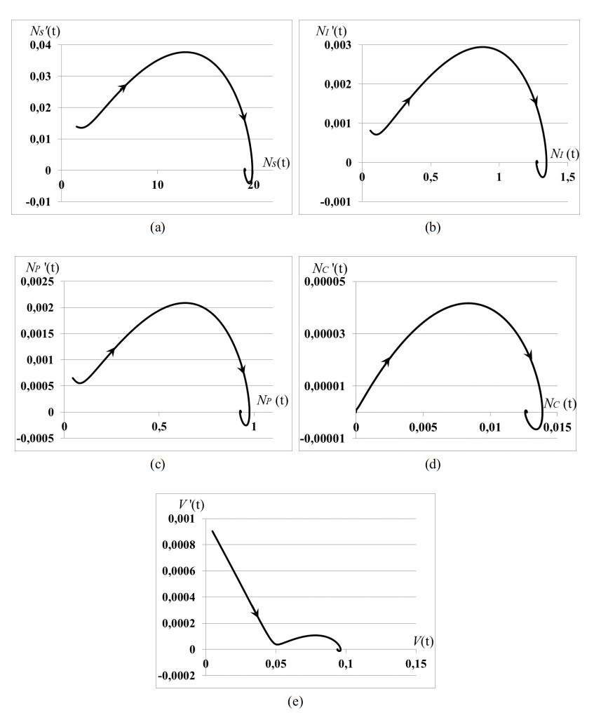
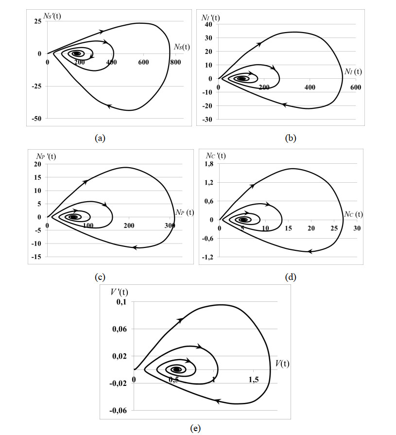
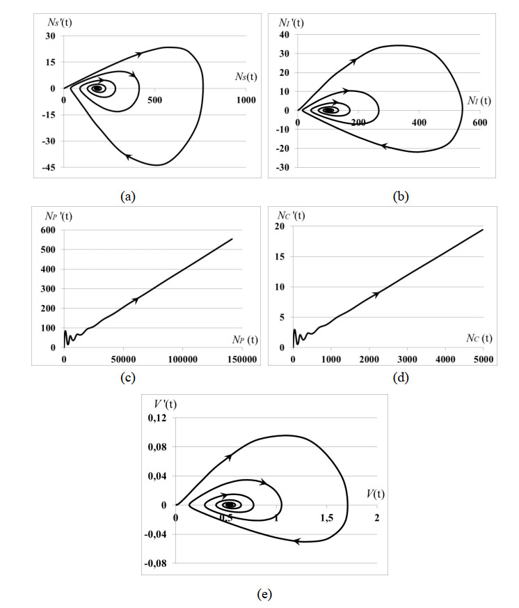
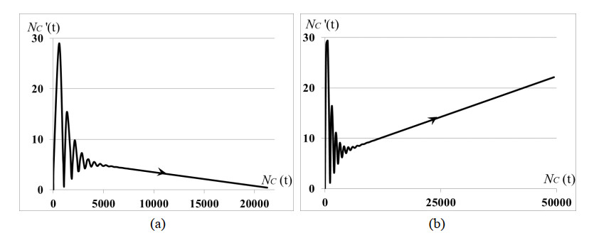
Stability analysis of an autonomous epidemic model of an age-structured sub-populations of susceptible, infected, precancerous and cancer cells and unstructured sub-population of human papilloma virus (HPV) (SIPCV epidemic model) aims to gain an insight into the features of cervical cancer disease. The model considers the immune functional response of organism to the virus population growing by the HPV-density dependent death rate, while the death rates of infected, precancerous and cancerous cells do not depend on the HPV quantity because the immune system of organism does not respond to its own cells. Interaction between susceptible cells and HPV is described by the Lotka-Voltera incidence rate and leads to the growth of infected cells. Some of infected cells become precancerous cells, and the other apoptosis when viruses leave infected cells and are ready to infect new susceptible cells. Precancerous cells partially become cancer cells with the density-dependent saturated rate. Conditions of existence of the endemic equilibrium of system were obtained. It was proved that this equilibrium is always locally asymptotically stable whenever it exists. We obtained: (i) the conditions of cancer tumor localization (asymptotically stable dynamical regimes), (ii) outbreak of cancer cell population (that may correspond to metastasis), (iii) outbreak of dysplasia (precancerous cells) which induces the outbreak of cancer cells (that may correspond to metastasis). In cases (ii), (iii) the conditions of existence of endemic equilibrium do not hold. All cases are illustrated by numerical experiments.
Citation: Vitalii V. Akimenko, Fajar Adi-Kusumo. Stability analysis of an age-structured model of cervical cancer cells and HPV dynamics[J]. Mathematical Biosciences and Engineering, 2021, 18(5): 6155-6177. doi: 10.3934/mbe.2021308
Stability analysis of an autonomous epidemic model of an age-structured sub-populations of susceptible, infected, precancerous and cancer cells and unstructured sub-population of human papilloma virus (HPV) (SIPCV epidemic model) aims to gain an insight into the features of cervical cancer disease. The model considers the immune functional response of organism to the virus population growing by the HPV-density dependent death rate, while the death rates of infected, precancerous and cancerous cells do not depend on the HPV quantity because the immune system of organism does not respond to its own cells. Interaction between susceptible cells and HPV is described by the Lotka-Voltera incidence rate and leads to the growth of infected cells. Some of infected cells become precancerous cells, and the other apoptosis when viruses leave infected cells and are ready to infect new susceptible cells. Precancerous cells partially become cancer cells with the density-dependent saturated rate. Conditions of existence of the endemic equilibrium of system were obtained. It was proved that this equilibrium is always locally asymptotically stable whenever it exists. We obtained: (i) the conditions of cancer tumor localization (asymptotically stable dynamical regimes), (ii) outbreak of cancer cell population (that may correspond to metastasis), (iii) outbreak of dysplasia (precancerous cells) which induces the outbreak of cancer cells (that may correspond to metastasis). In cases (ii), (iii) the conditions of existence of endemic equilibrium do not hold. All cases are illustrated by numerical experiments.

| [1] | P. J. Eifel, A. H. Klopp, J. S. Berek, P. A. Konstantinopoulos, Cancer of the cervix, vagina and vulva, in Cancer: Principles and Practice of Oncology (11th Edition), Wolters Kluwer, Philadelphia, (2019), 2083–2151. |
| [2] | B. L. Hoffman, J. O. Schorge, K. D. Bradshaw, L. M. Halvorson, J. I. Schaffer, M. M. Corton, Cervical cancer, in Williams gynecology (3rd Edition), McGraw-Hill, NY, 2016. |
| [3] | C. A. Kunos, F. W. Abdul-Karim, D. S. Dizon, R. Debernardo, Cervix uteri, in Principles and Practice of Gynecologic Oncology (7th Edition), Wolters Kluwer, Philadelphia, (2017), 946–983. |
| [4] | V. R. Martin, S. V. Temple, Cervical cancer, in Cancer Nursing: Principles and Practice (7th ed.), Jones and Bartlett Publishers, Sudbury Massachusetts, (2011), 1188–1204. |
| [5] | R. Smith, An age-structured model of human papillomavirus vaccination, Math. Comput. Simul., 82 (2011), 629–652. |
| [6] |
T. Malik, A. Gumel, E. Elbasha, Qualitative analysis of an age- and sex-structured vaccination model for human papillomavirus, Discrete Contin. Dynam. Syst. Ser. B, 18 (2013), 2151–2174. doi: 10.3934/dcdsb.2013.18.2151

|
| [7] | L. Aryati, T. S. Noor-Asih, F. Adi-Kusumo, M. S. Hardianti, Global stability of the disease free equilibrium in a cervical cancer model: a chance to recover, Far East J. Math. Sci., 103 (2018), 1535–1546. |
| [8] |
T. S. Noor-Asih, S. Lenhart, S. Wise, L. Aryati, F. Adi-Kusumo, M. S. Hardianti, et al., The dynamics of HPV infection and cervical cancer cells, Bull. Math. Biol., 78 (2016), 4–20. doi: 10.1007/s11538-015-0124-2
|
| [9] |
C. B. J. Woodman, S. I. Collins, L. S. Young, The natural history of cervical HPV infection: unresolved issues, Nat. Rev. Cancer, 7 (2007), 11–22. doi: 10.1038/nrc2050
|
| [10] |
F. Billy, J. Clairambault, F. Delaunay, C. Feillet, N. Robert, Age-structured cell population model to study the influence of growth factors on cell cycle dynamics, Math. Biosci. Eng., 10 (2013), 1–17. doi: 10.3934/mbe.2013.10.1
|
| [11] | F. Brauer, C. Castillo-Chavez, Mathematical Models in Population Biology and Epidemiology, Springer, New York, 2012. |
| [12] | O. Diekmann, J. A. P. Heesterbeek, Mathematical Epidemiology of Infectious diseases, John Wiley and Sons, Chichester, UK, 2000. |
| [13] |
J. Z. Farkas, G. F. Webb, Mathematical analysis of a clonal evolution model of tumour cell proliferation, J. Evol. Equations, 17 (2017), 275–308. doi: 10.1007/s00028-016-0369-8
|
| [14] |
A. Gandolfi, M. Iannelli, G. Marinoschi, An age-structured model of epidermis growth, J. Math. Biol., 62 (2011), 111–141. doi: 10.1007/s00285-010-0330-3
|
| [15] |
W. Krzyzanski, Pharmacodynamic models of age-structured cell populations, J. Pharmacokinet. Pharmacodyn., 42 (2015), 573–589. doi: 10.1007/s10928-015-9446-9
|
| [16] | J. Li, F. Brauer, Continuous-time age-structured models in population dynamics and epidemiology, in Mathematical Epidemiology, Springer, Berlin, (2008), 205–227. |
| [17] | X. Z. Li, J. Yang, M. Martcheva, Age Structured Epidemic Modelling, Springer, New York, 2020. |
| [18] | Z. Liu, J. Chen, J. Pang, ·P. Bi, S. Ruan, Modeling and analysis of a nonlinear age-structured model for tumour cell populations with quiescence. J. Nonlinear Sci., 28 (2018), 1763–1791. |
| [19] |
Z. Liu, C. Guo, H. Li, ·L. Zhao, Analysis of a nonlinear age-structured tumor cell population model, Nonlinear Dynam., 98 (2019), 283–300. doi: 10.1007/s11071-019-05190-4
|
| [20] |
Z. Liu, C. Guo, J. Yang, H. Li, Steady states analysis of a nonlinear age-structured tumor cell population model with quiescence and bidirectional transition, Acta Appl. Math., 169 (2020), 455–474. doi: 10.1007/s10440-019-00306-9
|
| [21] | M. Martcheva, An Introduction to Mathematical Epidemiology, Springer, New York, 2015. |
| [22] | J. Muller, Ch. Kuttler, Methods and Models in Mathematical Biology, Lecture Notes on Mathematical Modelling in Life Sciences, Springer, Berlin, 2015. |
| [23] | B. Perthame, Transport Equations in Biology (Frontiers in mathematics), Birkhauser Verlag, Basel, 2007. |
| [24] |
I. Roeder, M. Herberg, M. Horn, An "age"-structured model of hematopoietic stem cell organization with application to chronic myeloid leukaemia, Bull. Math. Biol., 71 (2009), 602–626. doi: 10.1007/s11538-008-9373-7
|
| [25] |
V. V. Akimenko, An age-structured SIR epidemic model with the fixed incubation period of infection, Comput. Math. Appl., 73 (2017), 1485–150. doi: 10.1016/j.camwa.2017.01.022
|
| [26] | F. M. Burnet, Intrinsic Mutagenesis: A Genetic Approach to Ageing, John Wiley & Sons Inc., New York, 1974. |
| [27] | L. M. Franks, M. A. Knowles, What is cancer? in Introduction to the Cellular and Molecular Biology of Cancer, Oxford University Press, Oxford, (2005), 21–44. |
| [28] |
K. Fernald, M. Kurokawa, Evading apoptosis in cancer, Trends Cell Biol., 23 (2013), 620–633. doi: 10.1016/j.tcb.2013.07.006
|
| [29] | V. V. Akimenko, Stability analysis of delayed age-structured resource-consumer model of population dynamics with saturated intake rate, Front. Ecol. Evol., 9 (2021), 1–15. |
| [30] |
V. V. Akimenko, R. Anguelov, Steady states and outbreaks of two-phase nonlinear age-structured model of population dynamics with discrete time delay, J. Biol. Dynam., 11 (2017), 75–101. doi: 10.1080/17513758.2016.1236988
|
| [31] |
V. V. Akimenko, V. Křivan, Asymptotic stability of delayed predator age-structured population models with an Allee effect, Math. Biosci., 306 (2018), 170–179. doi: 10.1016/j.mbs.2018.10.001
|
| [32] |
M. El-Doma, Analysis of an age-dependent SI epidemic model with disease-induced mortality and proportionate mixing assumption: the case of vertically transmitted diseases, J. Appl. Math., 2004 (2004) 235–253. doi: 10.1155/S1110757X0430118X
|
| [33] |
C. C. McCluskey, Global stability for an SEI epidemiological model with continuous age-structure in the exposed and infected classes, Math. Biosci. Eng., 9 (2012), 819–841. doi: 10.3934/mbe.2012.9.819
|
| [34] | Z. Zhang, S. Kumari, R. K. Upadhyay, A delayed e-epidemic SLBS model for computer virus, Adv. Differ. Equations, 1 (2019), 1–24. |
| [35] | R. Zhang, D. Li, S. Liu, Global analysis of an age-structured SEIR model with immigration of population and nonlinear incidence rate, J. Appl. Anal. Comput., 9 (2019), 1470–1492. |
| [36] | J. Yang, X. Wang, Existence of a non-autonomous SIR epidemic model with age structure, Adv. Differ. Equations, 2010 (2010), 1–23. |
| [37] |
Z. Yin, Y. Yu, Z. Lu, Stability analysis of an age-structured SEIRS model with time delay, Mathematics, 8 (2020), 455. doi: 10.3390/math8030455
|
Figures(4) / Tables(2)

Vitalii V. Akimenko, Fajar Adi-Kusumo. Stability analysis of an age-structured model of cervical cancer cells and HPV dynamics[J]. Mathematical Biosciences and Engineering, 2021, 18(5): 6155-6177. doi: 10.3934/mbe.2021308


 DownLoad: