Global stability mathematical analysis for virus transmission model with latent age structure

Shanjing Ren; Lingling Li; Shanjing Ren; Lingling Li

doi:10.3934/mbe.2022154

Mathematical Biosciences and Engineering

2022, Volume 19, Issue 4: 3337-3349. doi: 10.3934/mbe.2022154

Previous Article Next Article

Research article Special Issues

Global stability mathematical analysis for virus transmission model with latent age structure

Shanjing Ren ^{1
,
,},
Lingling Li ²

1.
School of Mathematics and Big Data, Guizhou Education University, Guiyang 550018, China
2.
School of Science, Xi'an Polytechnic University, Xi'an 710048, China

Academic Editor: Simon James Fong

Received: 29 November 2021 Revised: 10 January 2022 Accepted: 13 January 2022 Published: 24 January 2022

Background and objective
Mathematical model is a very important method for the control and prevention of disease transmissing. Based on the communication characteristics of diseases, it is necesssery to add fast and slow process into the model of infectious diseases, which more effectively shows the transmission mechanism of infectious diseases.
Methods
This paper proposes an age structure epidemic model with fast and slow progression. We analyze the model's dynamic properties by using the stability theory of differential equation under the assumption of constant population size.
Results
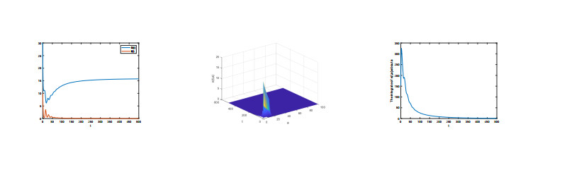
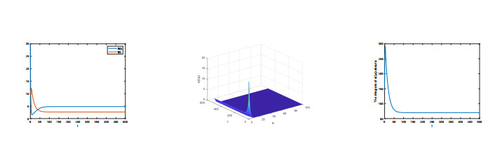
The very important threshold $ R_{0} $ was calculated. If $ R_{0} < 1 $, the disease-free equilibrium is globally asymptotically stable, whereas if $ R_{0} > 1 $, the Lyapunov function is used to show that endemic equilibrium is globally stable. Through more in-depth analysis for basic reproduction number, we obtain the greater the rate of slow progression of an infectious disease, the fewer the threshold results. In addition, we also provided some numerical simulations to prove our result.
Conclusions
Vaccines do not provide lifelong immunity, but can reduce the mortality of those infected. By vaccinating, the rate of patients entering slow progression increases and the threshold is correspondingly reduced. Therefore, vaccination can effectively control the transmission of Coronavirus. The theoretical incidence predicted by mathematical model can provide evidence for prevention and controlling the spread of the epidemic.
- age structure,
- Lyapunov function,
- infection equilibrium,
- global stability,
- prevention and control
Citation: Shanjing Ren, Lingling Li. Global stability mathematical analysis for virus transmission model with latent age structure[J]. Mathematical Biosciences and Engineering, 2022, 19(4): 3337-3349. doi: 10.3934/mbe.2022154

Related Papers:

Abstract

Background and objective

Mathematical model is a very important method for the control and prevention of disease transmissing. Based on the communication characteristics of diseases, it is necesssery to add fast and slow process into the model of infectious diseases, which more effectively shows the transmission mechanism of infectious diseases.

Methods

This paper proposes an age structure epidemic model with fast and slow progression. We analyze the model's dynamic properties by using the stability theory of differential equation under the assumption of constant population size.

Results

The very important threshold $ R_{0} $ was calculated. If $ R_{0} < 1 $, the disease-free equilibrium is globally asymptotically stable, whereas if $ R_{0} > 1 $, the Lyapunov function is used to show that endemic equilibrium is globally stable. Through more in-depth analysis for basic reproduction number, we obtain the greater the rate of slow progression of an infectious disease, the fewer the threshold results. In addition, we also provided some numerical simulations to prove our result.

Conclusions

Vaccines do not provide lifelong immunity, but can reduce the mortality of those infected. By vaccinating, the rate of patients entering slow progression increases and the threshold is correspondingly reduced. Therefore, vaccination can effectively control the transmission of Coronavirus. The theoretical incidence predicted by mathematical model can provide evidence for prevention and controlling the spread of the epidemic.

References

[1]	A. G. McKendrick, Application of mathematics to medical problems, in Proceedings of the Edinburgh Mathematical Society, 44 (1926), 98–130. https://doi.org/10.1017/S0013091500034428
[2]	W. O. Kermack, A. G. McKendrick, A contribution to the mathematical theory of epidemics, Proc. R. Soc. Lond. A, 115 (1927), 700–721. https://doi.org/10.1016/B978-0-12-802260-3.00004-3 doi: 10.1016/B978-0-12-802260-3.00004-3
[3]	F. Hoppensteadt, Mathematical Theories of Populations: Deomgraphics, Genetics, and Epidemics, SIAM, Philadelphia, 1975. https://doi.org/10.1137/1.9781611970487
[4]	M. Iannelli, Mathematical Theory of Age-structured Population Dynamics, Giardini Editori E Stampatori, Pisa, 1995.
[5]	G. F. Webb, Theory of Nonlinear Age-Dependent Population Dynamics, Marcel Dekker, New York, 1985.
[6]	S. Ren, Global stability in a tuberculosis model of imperfect treatment with age-dependent latency and relapse, Math. Biosci. Eng., 14 (2017), 1337–1360. https://doi.org/10.3934/mbe.2017069 doi: 10.3934/mbe.2017069
[7]	J. Wang, Z. Ran, T. Kuniya, A note on dynamics of an age-of-infection cholera model, Math. Biosci. Eng., 13 (2015), 227–247. https://doi.org/10.3934/mbe.2016.13.227 doi: 10.3934/mbe.2016.13.227
[8]	J. Wang, R. Zhang, T. Kuniya, The stability analysis of an SVEIR model with continuous age-structure in the exposed and infectious classes, J. Biol. Dyn., 9 (2015), 73–101. https://doi.org/10.1080/17513758.2015.1006696 doi: 10.1080/17513758.2015.1006696
[9]	S. Bentout, S. Djilali, A. Chekroun, Global threshold dynamics of an age structured alcoholism model, Int. J. Biomath., 14 (2021). https://doi.org/10.1142/S1793524521500133
[10]	G. F. Webb, A COVID-19 epidemic model predicting the effectiveness of vaccination, Infect. Dis. Rep., 13 (2021), 654–667. https://doi.org/10.3390/idr13030062 doi: 10.3390/idr13030062
[11]	B. Tang, X. Wang, Q. Li, N. L. Bragazzi, S. Tang, Y. Xiao, et al., Estimation of the transmission risk of the 2019-nCoV and its implication for public health interventions, J. Clin. Med., 9 (2020), 462. https://doi.org/10.3390/jcm9020462 doi: 10.3390/jcm9020462
[12]	J. Jiao, Z. Liu, S. Cai, Dynamics of an SEIR model with infectivity in incubation period and homestead-isolation on the susceptible, Appl. Math. Lett., 107 (2020), 106442. https://doi.org/10.1016/j.aml.2020.106442 doi: 10.1016/j.aml.2020.106442
[13]	Z. Tang, G. Zhao, T. Ouyang, Two-phase deep learning model for short-term wind direction forecasting, Renewable Energy, 173 (2021), 1005–1016. https://doi.org/10.1016/j.renene.2021.04.041 doi: 10.1016/j.renene.2021.04.041
[14]	C. C. McCluskey, Lyapunov functions for tuberculosis models with fast and slow progression, Math. Biosci. Eng., 3 (2016), 603–614. https://doi.org/10.3934/mbe.2006.3.603 doi: 10.3934/mbe.2006.3.603
[15]	V. Capasso, G. Serio, A generalization of the Kermack-McKendrick deterministic epidemic model, Math. Biosci., 42 (1978), 43–61. https://doi.org/10.1016/0025-5564(78)90006-8 doi: 10.1016/0025-5564(78)90006-8
[16]	P. Magal, Compact attractors for time-periodic age-structured population models, Electron. J. Differ. Equations, 65 (2001), 229–262. https://doi.org/10.1023/A:1011257222927 doi: 10.1023/A:1011257222927
[17]	P. Magal, H. R. Thieme, Eventual compactness for semiflows generated by nonlinear age-structured models, Commun. Pure Appl. Anal., 3 (2004), 695–727. https://doi.org/10.3934/cpaa.2004.3.695 doi: 10.3934/cpaa.2004.3.695
[18]	R. D. Demasse, A. Ducrot, An age-structured within-host model for multistrain malaria infections, SIAM J. Appl. Math., 73 (2013), 572–593. https://doi.org/10.1137/120890351 doi: 10.1137/120890351
[19]	F. Brauer, Z. Shuai, P. van den Driessche, Dynamics of an age-of-infection cholera model, Math. Biosci. Eng., 10 (2013), 1335–1349. https://doi.org/10.3934/mbe.2013.10.1335 doi: 10.3934/mbe.2013.10.1335

Reader Comments

Your name:*

Email:*
© 2022 the Author(s), licensee AIMS Press. This is an open access article distributed under the terms of the Creative Commons Attribution License (http://creativecommons.org/licenses/by/4.0)