A simple model of cardiac mitochondrial respiration with experimental validation

Bachar Tarraf; Emmanuel Suraniti; Camille Colin; Stéphane Arbault; Philippe Diolez; Michael Leguèbe; Yves Coudière; Bachar Tarraf; Emmanuel Suraniti; Camille Colin; Stéphane Arbault; Philippe Diolez; Michael Leguèbe; Yves Coudière

doi:10.3934/mbe.2021291

Mathematical Biosciences and Engineering

2021, Volume 18, Issue 5: 5758-5789. doi: 10.3934/mbe.2021291

Previous Article Next Article

Research article Special Issues

A simple model of cardiac mitochondrial respiration with experimental validation

1.
Inria Bordeaux-Sud-Ouest, team CARMEN, Talence, France
2.
IHU Liryc, Fondation Bordeaux Université, Pessac, France
3.
Institut de Mathématiques de Bordeaux, UMR CNRS 5251, Talence, France
4.
Université de Bordeaux, Bordeaux, France
5.
ISM, CNRS UMR 5255, Bordeaux, France
6.
INSERM, Centre de Recherche Cardio-Thoracique de Bordeaux, U-1045, Bordeaux, France

Received: 12 February 2021 Accepted: 06 June 2021 Published: 25 June 2021

Cardiac mitochondria are intracellular organelles that play an important role in energy metabolism and cellular calcium regulation. In particular, they influence the excitation-contraction cycle of the heart cell. A large number of mathematical models have been proposed to better understand the mitochondrial dynamics, but they generally show a high level of complexity, and their parameters are very hard to fit to experimental data.

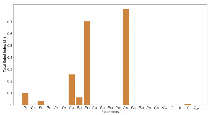
We derived a model based on historical free energy-transduction principles, and results from the literature. We proposed simple expressions that allow to reduce the number of parameters to a minimum with respect to the mitochondrial behavior of interest for us. The resulting model has thirty-two parameters, which are reduced to twenty-three after a global sensitivity analysis of its expressions based on Sobol indices.

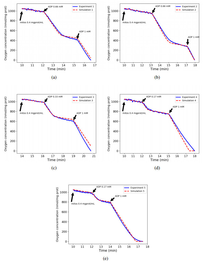
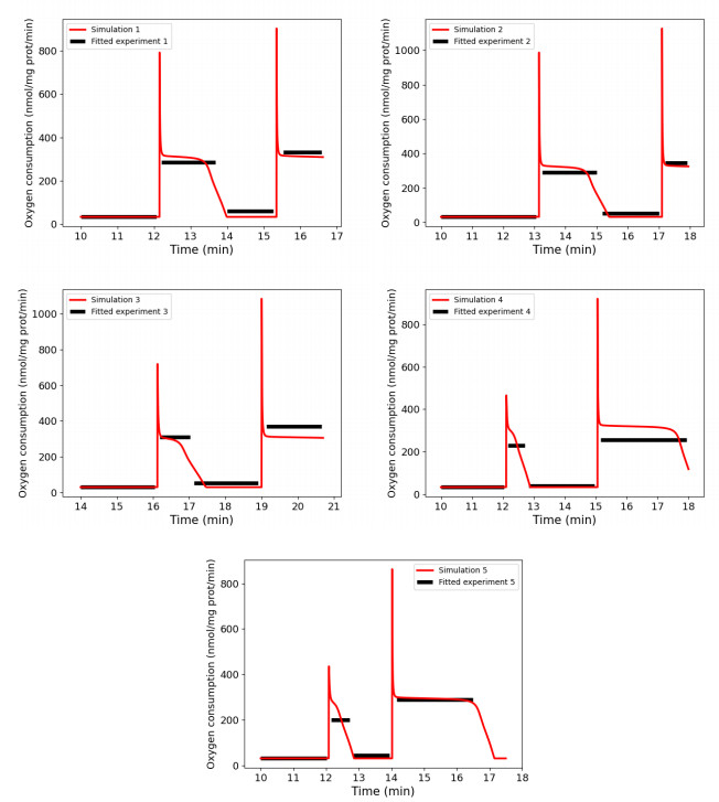
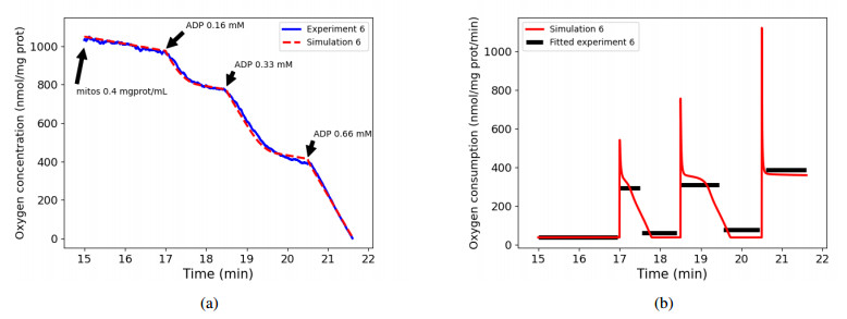
We calibrated our model to experimental data that consists of measurements of mitochondrial respiration rates controlled by external ADP additions. A sensitivity analysis of the respiration rates showed that only seven parameters can be identified using these observations. We calibrated them using a genetic algorithm, with five experimental data sets. At last, we used the calibration results to verify the ability of the model to accurately predict the values of a sixth dataset.

Results show that our model is able to reproduce both respiration rates of mitochondria and transitions between those states, with very low variability of the parameters between each experiment. The same methodology may apply to recover all the parameters of the model, if corresponding experimental data were available.

Keywords:

Citation: Bachar Tarraf, Emmanuel Suraniti, Camille Colin, Stéphane Arbault, Philippe Diolez, Michael Leguèbe, Yves Coudière. A simple model of cardiac mitochondrial respiration with experimental validation[J]. Mathematical Biosciences and Engineering, 2021, 18(5): 5758-5789. doi: 10.3934/mbe.2021291

Related Papers:

[1]	Ahmet Sinan Cevik, Ismail Naci Cangul, Yilun Shang . Matching some graph dimensions with special generating functions. AIMS Mathematics, 2025, 10(4): 8446-8467. doi: 10.3934/math.2025389
[2]	Dalal Awadh Alrowaili, Uzma Ahmad, Saira Hameeed, Muhammad Javaid . Graphs with mixed metric dimension three and related algorithms. AIMS Mathematics, 2023, 8(7): 16708-16723. doi: 10.3934/math.2023854
[3]	Yuni Listiana, Liliek Susilowati, Slamin Slamin, Fadekemi Janet Osaye . A central local metric dimension on acyclic and grid graph. AIMS Mathematics, 2023, 8(9): 21298-21311. doi: 10.3934/math.20231085
[4]	Ahmed Alamer, Hassan Zafar, Muhammad Javaid . Study of modified prism networks via fractional metric dimension. AIMS Mathematics, 2023, 8(5): 10864-10886. doi: 10.3934/math.2023551
[5]	Supachoke Isariyapalakul, Witsarut Pho-on, Varanoot Khemmani . The true twin classes-based investigation for connected local dimensions of connected graphs. AIMS Mathematics, 2024, 9(4): 9435-9446. doi: 10.3934/math.2024460
[6]	Abdessatar Souissi, El Gheteb Soueidy, Mohamed Rhaima . Clustering property for quantum Markov chains on the comb graph. AIMS Mathematics, 2023, 8(4): 7865-7880. doi: 10.3934/math.2023396
[7]	Hashem Bordbar, Sanja Jančič-Rašovič, Irina Cristea . Regular local hyperrings and hyperdomains. AIMS Mathematics, 2022, 7(12): 20767-20780. doi: 10.3934/math.20221138
[8]	S. Gajavalli, A. Berin Greeni . On strong geodeticity in the lexicographic product of graphs. AIMS Mathematics, 2024, 9(8): 20367-20389. doi: 10.3934/math.2024991
[9]	Xia Hong, Wei Feng . Completely independent spanning trees in some Cartesian product graphs. AIMS Mathematics, 2023, 8(7): 16127-16136. doi: 10.3934/math.2023823
[10]	Chenggang Huo, Humera Bashir, Zohaib Zahid, Yu Ming Chu . On the 2-metric resolvability of graphs. AIMS Mathematics, 2020, 5(6): 6609-6619. doi: 10.3934/math.2020425

Abstract

1. Introduction

Fractional calculus is a modification of the notion of differentiation and integration of arbitrary orders ^{[1,2,3,4,5,6,7]}. As there exist various prototypes in engineering and sciences, fractional calculus has attained the researcher's interest. Multiple models in numerous aspects such as; physics, biology, and engineering are tackled as per fractional differential and integral calculus. Some examples are electrochemistry, signal processing, diffusion, finance, acoustic, plasma physics, image processing, and others ^{[8,9,10,11,12,13]}.

Integral transforms are notified as one of the most suitable approaches to tackle models regarding applied mathematics, mathematical physics, engineering, and some other branches as well. The primary motivation is to deal with the provided mathematical model via any suitable integral transform and to retrieve the associated outcome in the best possible approach.

Via an appropriate selection of integral transform, the differential and integral equations can be transformed into an algebraic equations system, which can be easily tackled.

Various integral transforms and integral transform-based approaches are generated and incorporated for this purpose, such as; Laplace transform ^[14], Sumudu transform ^[15], Elzaki transform ^[16], and Natural transform ^[17], and many others.

Definition 1: Shehu transform of the function $\theta \left(\tau \right)$ is defined over the following functions ^[18,19,20].

$A = \left\{\epsilon \left(\tau \right):there\;exists\;N, {k}_{1}, {k}_{2} > 0\;s.t.\;\left|\theta \left(\tau \right)\right| < Nexp\left(\frac{\left|\tau \right|}{{k}_{i}}\right),\; where\;\tau \in {\left(-1\right)}^{j}\times [0, \infty )\right\}.$

(1)

Definition 2: Shehu transform of function $\epsilon \left(\tau \right)$ is defined as follows ^[18,19,20]:

$S\left[\epsilon \left(\tau \right)\right] = F\left[s, u\right] = {\int }_{0}^{\infty }exp\left[-\frac{s\tau }{u}\right]\epsilon \left(\tau \right)d\tau .$

(2)

Definition 3: Inverse Shehu transform is defined as follows ^[18,19,20]:

${S}^{-1}\left[F\left(s, u\right)\right] = \epsilon \left(\tau \right).$

(3)

Where $s$ , $u$ are the Shehu transform variables. $\alpha \in R$ .

Definition 4: ^[18,19,20]

$S\left[{\epsilon }^{{'}}\left(\tau \right)\right] = \frac{s}{u}F\left[s, u\right]-\epsilon \left(0\right) ,$

(4)

$S\left[{\epsilon }^{{'}{'}}\left(\tau \right)\right] = \frac{{s}^{2}}{{u}^{2}}F\left(s, u\right)-\frac{s}{u}\epsilon \left(0\right)-\epsilon {'}\left(0\right) ,$

(5)

$S\left[{\epsilon }^{{'}{'}{'}}\left(\tau \right)\right] = \frac{{s}^{3}}{{u}^{3}}F\left[s, u\right]-\frac{{s}^{2}}{{u}^{2}}\epsilon \left(0\right)-\frac{s}{u}{\epsilon }^{{'}}\left(0\right)-\epsilon {'}{'}\left(0\right) .$

(6)

Definition 5: Linearity property of Shehu transform ^[18,19,20]:

$S\left[{c}_{1}{\epsilon }_{1}\left(\tau \right)+{c}_{2}{\epsilon }_{2}\left(\tau \right)\right] = {c}_{1}S\left[{\epsilon }_{1}\left(\tau \right)\right]+{c}_{2}S\left[{\epsilon }_{2}\left(\tau \right)\right] .$

(7)

Definition 6: Linearity property of inverse Shehu transform ^[18,19,20]:

${\epsilon }_{1}\left(\tau \right) = {S}^{-1}\left[{F}_{1}\right(s, u\left)\right]\; {\rm{and}} \; {\epsilon }_{2}\left(\tau \right) = {S}^{-1}\left[{F}_{2}\right(s, u\left)\right] ,$

then

${S}^{-1}\left[{c}_{1}{F}_{1}(s, u)+{c}_{2}{F}_{2}(s, u)\right] = {c}_{1}{S}^{-1}\left[{F}_{1}(s, u)\right]+{c}_{2}{S}^{-1}\left[{F}_{2}(s, u)\right],$

${S}^{-1}\left[{c}_{1}{F}_{1}(s, u)+{c}_{2}{F}_{2}(s, u)\right] = {c}_{1}{\epsilon }_{1}\left(\tau \right)+{c}_{2}{\epsilon }_{2}\left(\tau \right) .$

Definition 7: Shehu transform of Caputo fractional derivative [C.F.D.] ^[20,21]:

$S\left[{D}_{t}^{\alpha }\epsilon \left(\mu , \tau \right)\right] = \frac{{s}^{\alpha }}{{\nu }^{\alpha }}S\left[\epsilon \left(\mu , \tau \right)\right]-{\sum }_{r = 0}^{\theta -1}{\left(\frac{s}{\nu }\right)}^{\alpha -r-1}{\epsilon }^{r}\left(\mu , 0\right).$

(8)

Definition 8: Mittag-Leffler function considered for two parameters was given in ^[22,23,24].

${E}_{\mu , \nu }\left(n\right) = {\sum }_{k = 0}^{\infty }\frac{{n}^{k}}{\mathrm{\Gamma }(k\mu +\nu )} .$

(9)

Where ${E}_{\mathrm{1, 1}}\left(n\right) = \mathrm{e}\mathrm{x}\mathrm{p}\left(n\right)$ and ${E}_{\mathrm{2, 1}}\left({n}^{2}\right) = \mathrm{c}\mathrm{o}\mathrm{s}\left(n\right)$ .

In Tables 1 and 2 basic formulae regarding Shehu transform and inverse Shehu transform are provided.

Table 1. Chart regarding to the Shehu transform ^[20].

	$\mathit{\boldsymbol{\epsilon }}\left(\mathit{\boldsymbol{\tau }}\right)$	$\mathit{\boldsymbol{S}}\left[\mathit{\boldsymbol{\epsilon }}\right(\mathit{\boldsymbol{\tau }}\left)\right]=\mathit{\boldsymbol{F}}(\mathit{\boldsymbol{s}}, \mathit{\boldsymbol{\nu }})$
1.	$1$	$\frac{\nu }{s}$
2.	$\tau$	$\frac{{\nu }^{2}}{{s}^{2}}$
3.	${\tau }^{m}, m\in N$	$\angle m{\left(\frac{\nu }{s}\right)}^{m+1}$
4.	${\tau }^{m}, m > -1$	$\mathrm{\Gamma }(m+1){\left(\frac{\nu }{s}\right)}^{m+1}$
5.	${e}^{a\tau }$	$\frac{\nu }{s-a\nu }$
6.	$\mathrm{s}\mathrm{i}\mathrm{n}\left(m\tau \right)$	$\frac{m{\nu }^{2}}{{s}^{2}+{m}^{2}{\nu }^{2}}$
7.	$cos\left(m\tau \right)$	$\frac{s{\nu }^{2}}{{s}^{2}+{m}^{2}{\nu }^{2}}$
8.	$sinh\left(m\tau \right)$	$\frac{m{\nu }^{2}}{{s}^{2}-{m}^{2}{\nu }^{2}}$
9.	$cosh\left(m\tau \right)$	$\frac{s{\nu }^{2}}{{s}^{2}-{m}^{2}{\nu }^{2}}$

| Show Table

DownLoad: CSV

Table 2. Chart regarding to the inverse Shehu transform ^[20].

	$\mathit{\boldsymbol{F}}(\mathit{\boldsymbol{s}}, \mathit{\boldsymbol{\nu }})$	$\mathit{\boldsymbol{\epsilon }}\left(\mathit{\boldsymbol{\tau }}\right)={\mathit{\boldsymbol{S}}}^{{\bf{-1}}}\left[\mathit{\boldsymbol{F}}\right(\mathit{\boldsymbol{s}}, \mathit{\boldsymbol{\nu }}\left)\right]$
1.	$\frac{\nu }{s}$	$1$
2.	$\frac{{\nu }^{2}}{{s}^{2}}$	$\tau$
3.	${\left(\frac{\nu }{s}\right)}^{m+1}$	$\frac{{\tau }^{m}}{\angle m}$
4.	$\mathrm{\Gamma }(m+1){\left(\frac{\nu }{s}\right)}^{m+1}$	$\frac{{\tau }^{m}}{\mathrm{\Gamma }(m+1)}$
5.	$\frac{\nu }{s-a\nu }$	${e}^{a\tau }$
6.	$\frac{m{\nu }^{2}}{{s}^{2}+{m}^{2}{\nu }^{2}}$	$\mathrm{s}\mathrm{i}\mathrm{n}\left(m\tau \right)$
7.	$\frac{s{\nu }^{2}}{{s}^{2}+{m}^{2}{\nu }^{2}}$	$cos\left(m\tau \right)$
8.	$\frac{m{\nu }^{2}}{{s}^{2}-{m}^{2}{\nu }^{2}}$	$sinh\left(m\tau \right)$
9.	$\frac{s{\nu }^{2}}{{s}^{2}-{m}^{2}{\nu }^{2}}$	$cosh\left(m\tau \right)$

| Show Table

DownLoad: CSV

${\bf{1}}\mathit{\boldsymbol{D}}$ Non-linear time-fractional Schrödinger equation.

$i{D}_{t}^{\alpha }\theta \left(\mu , \tau \right) = R\left[\theta \left(\mu , \tau \right)\right]+N\left[\theta \left(\mu , \tau \right)\right]+\phi \left(\mu , \tau \right).$

(10)

${\bf{2}}\mathit{\boldsymbol{D}}$ Non-linear time-fractional Schrödinger equation.

$i{D}_{t}^{\alpha }\theta ({\mu }_{1}, {\mu }_{2}, \tau ) = R\left[\theta \left({\mu }_{1}, {\mu }_{2}, \tau \right)\right]+N\left[\theta \left({\mu }_{1}, {\mu }_{2}, \tau \right)\right]+\phi ({\mu }_{1}, {\mu }_{2}, \tau ) .$

(11)

${\bf{3}}\mathit{\boldsymbol{D}}$ Non-linear time-fractional Schrödinger equation.

$i{D}_{t}^{\alpha }\theta \left({\mu }_{1}, {\mu }_{2}, {\mu }_{3}, \tau \right) = R\left[\theta \left({\mu }_{1}, {\mu }_{2}, {\mu }_{3}, \tau \right)\right]+N\left[\theta \left({\mu }_{1}, {\mu }_{2}, {\mu }_{3}, \tau \right)\right]+\phi \left({\mu }_{1}, {\mu }_{2}, {\mu }_{3}, \tau \right).$

(12)

One of the well-known models in mathematical physics is Schr $\ddot{o}$ dinger equation model. There exist various implementations in numerous branches, such as; non-linear optics ^[25], mean-field theory of Bose-Einstein condensates ^[26,27], and plasma physics ^[28]. One emerging aspect of quantum physics is considered as fractional Schr $\ddot{o}$ dinger equation; which is associated with the notion of non-local quantum phenomena.

Naber ^[29] notified time-fractional Schr $\ddot{o}$ dinger equation regarding Caputo derivative. Wang and Xu ^[30] elaborated on the linear Schr $\ddot{o}$ dinger equation regarding the space-fractional and time-fractional aspects as well as tackled the models via integral transform approach. Due to the existence of numerous implementations of the time-fractional Schr $\ddot{o}$ dinger equation; various researchers have worked in this field. Regarding this, novel analytical and numerical regimes have been generated for the time-fractional Schr $\ddot{o}$ dinger equation ^{[31,32,33,34]}. Hemida et al. ^[35] implemented HAM to provide the approximated results for the space-time fractional Schr $\ddot{o}$ dinger equation. More work related to fractional Schr $\ddot{o}$ dinger equation is provided in ^[36,37,38]. Other noteworthy work in this regard is notified as ^{[39,40,41,42]}.

The main advantage of ADM is that it does not rely upon perturbation or linearization or any discretization. Therefore, the actual outcome of the model remains unchanged. Discretization of variables is not demanded, which is a difficult and challenging approach. It means that the obtained results are error-free, which occurred because of discretization. Furthermore, it is accurate in finding the approximated and exact solutions of the non-linear prototypes. Such methods can be implemented to the diversified differential equations such as; integro-differential equations, differential-algebraic equations, differential-difference equations, as well as some functional equations, eigenvalue problems, and Stochastic system problems.

The main idea of the present study is to concentrate on the implementation of Shehu ADM for attaining the exact solution to the Schr $\ddot{o}$ dinger equations in various dimensions. Some latest research regarding this field is provided on ^{[43,44,45,46,47]}.

Novelty and significance of the paper

There are several schemes observed in the literature that deal with fractional Schr $\ddot{o}$ dinger equation in one, two, or three dimensions, but rare methods are provided that tackles fractional Schr $\ddot{o}$ dinger equation in all one, two, and three dimensions. Therefore, the authors have focused on developing a technique that proves the validity of the approximated-analytical solution of the mentioned equations in one, two, and three dimensions.

An iterative scheme is developed in the present research regarding the solution of fractional Schr $\ddot{o}$ dinger equation in one, two, and three dimensions. The present scheme is easy to implement and needs no complex programming regarding numerical discretization. Developing the numerical programs for the fractional PDEs is not an easy task; therefore, developing such iterative schemes is the need of time to find the approximated-analytical solutions. There exist several transforms provided in the literature, but from the calculation aspect, some transforms are easy to implement, and some are not. Shehu ADM is noticed as one of the easiest methods to implement integral transform among all existing integral transforms; as in the case of Shehu ADM, no perturbation parameter is required. Via literature, it is observed that fractional Schrödinger equations have never been solved in one, two, and three dimensions with the aid of a single integral transform. Therefore, due to the importance of such equations, in this research, concentration is focused upon the solution for the same, which retains the novelty of the study. Furthermore, convergence analyses are also incorporated in the article.

Motivation of the study

In the present research, an iterative regime is developed and incorporated named Shehu ADM regarding the solution of fractional Schr $\ddot{o}$ dinger equation in one, two, and three dimensions. The present regime is easy to implement and needs no complex calculation in the process of numerical discretization. Generating the numerical programs to deal with the fractional PDEs is cumbersome; therefore, generating such novel iterative regimes is demanded to fetch the approximated-analytical solutions.

There exist numerous transforms in the literature, but as per the calculation aspect, some transforms are easy to incorporate, but some are not. Shehu transform ADM is notified as one of the easiest methods. From an exploration of the literature, it is noticed that fractional Schrödinger equations are rarely solved in one, two, and three dimensions with the aid of a single integral transform-based method. Therefore, in this research, the focus is on finding the solution for the same, which contains the novelty of the research. Moreover, error analysis and convergence analysis are also elaborated in this article.

In the present paper, the convergence of the method is checked numerically. Convergence is affirmed via Tables 3–. As per –, it is observed that on increasing the number of grid points the ${L}_{\infty }$ error norm got reduced rapidly, which is robust proof of the convergence of the generated semi-analytical techniques.

Table 3. Comparison of

${L}_{\infty }$ errors at different time levels regarding Example 1.

$\mathit{\boldsymbol{N}}$	${\mathit{\boldsymbol{L}}}_{{\infty }}$ at $\mathit{\boldsymbol{t}}$ =1	${\mathit{\boldsymbol{L}}}_{{\infty }}$ at $\mathit{\boldsymbol{t}}$ =2	${\mathit{\boldsymbol{L}}}_{{\infty }}$ at $\mathit{\boldsymbol{t}}$ =3
11	2.4979e-08	5.0711e-05	4.3236e-03
21	4.4755e-16	4.1023e-14	2.0302e-10
31	4.4755e-16	5.6610e-16	1.3911e-15
	Convergence up to ${{\bf{10}}}^{{\bf{-16}}}$	Convergence up to ${{\bf{10}}}^{{\bf{-16}}}$	Convergence up to ${{\bf{10}}}^{{\bf{-16}}}$

| Show Table

DownLoad: CSV

Table 4. Comparison of

${L}_{\infty }$ errors at different time levels regarding Example 2.

$\mathit{\boldsymbol{N}}$	${\mathit{\boldsymbol{L}}}_{\mathit{\boldsymbol{\infty }}}$ at $\mathit{\boldsymbol{t}}$ =0.1	${\mathit{\boldsymbol{L}}}_{\mathit{\boldsymbol{\infty }}}$ at $\mathit{\boldsymbol{t}}$ =0.2	${\mathit{\boldsymbol{L}}}_{\mathit{\boldsymbol{\infty }}}$ at $\mathit{\boldsymbol{t}}$ =0.3
11	7.8430e-09	1.5949e-05	1.3635e-03
21	2.4825e-16	4.8963e-15	2.2250e-11
31	3.7238e-16	5.5788e-16	1.1802e-15
	Convergence up to ${{\bf{10}}}^{{\bf{-16}}}$	Convergence up to ${{\bf{10}}}^{{\bf{-16}}}$	Convergence up to ${{\bf{10}}}^{{\bf{-15}}}$

| Show Table

DownLoad: CSV

Table 5. Comparison of

${L}_{\infty }$ errors at different time levels regarding Example 3.

$\mathit{\boldsymbol{N}}$	${\mathit{\boldsymbol{L}}}_{\mathit{\boldsymbol{\infty }}}$ at $\mathit{\boldsymbol{t}}$ =1.0	${\mathit{\boldsymbol{L}}}_{\mathit{\boldsymbol{\infty }}}$ at $\mathit{\boldsymbol{t}}$ =1.3	${\mathit{\boldsymbol{L}}}_{\mathit{\boldsymbol{\infty }}}$ at $\mathit{\boldsymbol{t}}$ =1.5
21	3.1906e-07	7.8034e-05	1.5627e-03
31	8.4843e-15	7.0869e-12	5.9702e-10
41	6.4393e-15	2.9407e-14	5.6576e-14
	Convergence up to ${{\bf{10}}}^{{\bf{-15}}}$	Convergence up to ${{\bf{10}}}^{{\bf{-14}}}$	Convergence up to ${{\bf{10}}}^{{\bf{-14}}}$

| Show Table

DownLoad: CSV

Table 6. Comparison of

${L}_{\infty }$ errors at different time levels regarding Example 4.

$\mathit{\boldsymbol{N}}$	${\mathit{\boldsymbol{L}}}_{\mathit{\boldsymbol{\infty }}}$ at $\mathit{\boldsymbol{t}}$ =1.0	${\mathit{\boldsymbol{L}}}_{\mathit{\boldsymbol{\infty }}}$ at $\mathit{\boldsymbol{t}}$ =1.3	${\mathit{\boldsymbol{L}}}_{\mathit{\boldsymbol{\infty }}}$ at $\mathit{\boldsymbol{t}}$ =1.5
11	1.8114e-06	3.2318e-05	1.5541e-04
21	1.3092e-16	2.0510e-14	4.0767e-13
31	2.2377e-16	2.4825e-16	2.4825e-16
	Convergence up to ${{\bf{10}}}^{{\bf{-16}}}$	Convergence up to ${{\bf{10}}}^{{\bf{-16}}}$	Convergence up to ${{\bf{10}}}^{{\bf{-16}}}$

| Show Table

DownLoad: CSV

Table 7. Comparison of

${L}_{\infty }$ errors at different time levels regarding Example 5.

$\mathit{\boldsymbol{N}}$	${\mathit{\boldsymbol{L}}}_{\mathit{\boldsymbol{\infty }}}$ at $\mathit{\boldsymbol{t}}$ =1	${\mathit{\boldsymbol{L}}}_{\mathit{\boldsymbol{\infty }}}$ at $\mathit{\boldsymbol{t}}$ =2	${\mathit{\boldsymbol{L}}}_{\mathit{\boldsymbol{\infty }}}$ at $\mathit{\boldsymbol{t}}$ =3
21	4.0910e-14	8.4807e-08	4.1536e-04
31	3.3766e-16	1.9860e-15	1.5697e-10
41	3.3766e-16	1.7342e-15	1.6577e-14
	Convergence up to ${{\bf{10}}}^{{\bf{-16}}}$	Convergence up to ${{\bf{10}}}^{{\bf{-15}}}$	Convergence up to ${{\bf{10}}}^{{\bf{-14}}}$

| Show Table

DownLoad: CSV

Table 8. Comparison of

${L}_{\infty }$ errors at different time levels regarding Example 6.

$\mathit{\boldsymbol{N}}$	${\mathit{\boldsymbol{L}}}_{\mathit{\boldsymbol{\infty }}}$ at $\mathit{\boldsymbol{t}}$ =1	${\mathit{\boldsymbol{L}}}_{\mathit{\boldsymbol{\infty }}}$ at $\mathit{\boldsymbol{t}}$ =2	${\mathit{\boldsymbol{L}}}_{\mathit{\boldsymbol{\infty }}}$ at $\mathit{\boldsymbol{t}}$ =3
21	4.4168e-13	9.1039e-07	4.4156e-03
31	5.7220e-17	5.5268e-14	1.5682e-08
41	4.6548e-17	6.9573e-16	8.8374e-15
	Convergence up to ${{\bf{10}}}^{{\bf{-17}}}$	Convergence up to ${{\bf{10}}}^{{\bf{-16}}}$	Convergence up to ${{\bf{10}}}^{{\bf{-15}}}$

| Show Table

DownLoad: CSV

2. Outline of the paper

● The present paper is divided into different sections and subsections.

● In Section 3, Implementation of the Shehu ADM is developed for various kinds of fractional Schr $\ddot{o}$ dinger equations.

● In Sub-section 3.1, the general formula is generated for $1D$ time-fractional Schrödinger equation.

● In Sub-section 3.2, the general formula is generated for $2D$ time-fractional Schrödinger equation.

● In Sub-section 3.3, the general formula is generated for $3D$ time-fractional Schrödinger equation.

● In Section 4, six examples are elaborated to validate the efficiency and efficacy of the developed regime.

● In Section 5, graphical analysis, error analysis, and convergence analysis is notified.

● Section 6 is provided as the concluding remarks.

3. Implementation of the proposed regime

3.1. Implementation of the scheme on $1{D}$ time-fractional Schr $\ddot{{o}}$ dinger equation

Applying Shehu transform upon Eq (1):

$\begin{array}{l} iS\left[{D}_{\tau }^{\alpha }\theta \left(\mu , \tau \right)\right] = S\left[R\left[\theta \left(\mu , \tau \right)\right]+N\left[\theta \left(\mu , \tau \right)\right]+\phi \left(\mu , \tau \right)\right] \\ \Rightarrow S\left[{D}_{\tau }^{\alpha }\theta \left(\mu , \tau \right)\right] = -iS\left[R\left[\theta \left(\mu , \tau \right)\right]+N\left[\theta \left(\mu , \tau \right)\right]+\phi \left(\mu , \tau \right)\right]\\ {\Rightarrow \left(\frac{s}{\nu }\right)}^{\alpha }S\left[\theta \left(\mu , \tau \right)\right]-\sum\limits_{r = 0}^{\theta -1}{\left(\frac{s}{\nu }\right)}^{\alpha -r-1}{\theta }^{r}\left(\mu , 0\right) = -iS\left[R\left[\theta \left(\mu , \tau \right)\right]+N\left[\theta \left(\mu , \tau \right)\right]+\phi \left(\mu , \tau \right)\right] \\ {\Rightarrow \left(\frac{s}{\nu }\right)}^{\alpha }S\left[\theta \left(\mu , \tau \right)\right] = \sum\limits_{r = 0}^{\theta -1}{\left(\frac{s}{\nu }\right)}^{\alpha -r-1}{\theta }^{r}\left(\mu , 0\right)-iS\left[R\left[\theta \left(\mu , \tau \right)\right]+N\left[\theta \left(\mu , \tau \right)\right]+\phi \left(\mu , \tau \right)\right] \\ \Rightarrow S\left[\theta \left(\mu , \tau \right)\right] = {\left(\frac{\nu }{s}\right)}^{\alpha }\sum\limits_{r = 0}^{\theta -1}{\left(\frac{s}{\nu }\right)}^{\alpha -r-1}{\theta }^{r}\left(\mu , 0\right)-i{\left(\frac{\nu }{s}\right)}^{\alpha }S\left[R\left[\theta \left(\mu , \tau \right)\right]+N\left[\theta \left(\mu , \tau \right)\right]+\phi \left(\mu , \tau \right)\right] \\ \Rightarrow \theta \left(\mu , \tau \right) = {S}^{-1}\left[{\left(\frac{\nu }{s}\right)}^{\alpha }\sum\limits_{r = 0}^{\theta -1}{\left(\frac{s}{\nu }\right)}^{\alpha -r-1}{\theta }^{r}\left(\mu , 0\right)\right]-i{S}^{-1}\left[{\left(\frac{\nu }{s}\right)}^{\alpha }S\left[R\left[\theta \left(\mu , \tau \right)\right]+N\left[\theta \left(\mu , \tau \right)\right]+\phi \left(\mu , \tau \right)\right]\right] \\ \Rightarrow \sum\limits_{n = 0}^{\infty }{\theta }_{n}(\mu , \tau ) = {S}^{-1}\left[{\left(\frac{\nu }{s}\right)}^{\alpha }\sum\limits_{r = 0}^{\theta -1}{\left(\frac{s}{\nu }\right)}^{\alpha -r-1}{\theta }^{r}\left(\mu , 0\right)+\phi \left(\mu , \tau \right)\right] \\ \;\;\;\;\;\;\;\;\;\; -i{S}^{-1}\left[{\left(\frac{\nu }{s}\right)}^{\alpha }S\left[R\left[{\sum }_{n = 0}^{\infty }{\theta }_{n}(\mu , \tau )\right]+N\left[{\sum }_{n = 0}^{\infty }{\theta }_{n}(\mu , \tau )\right]\right]\right] . \end{array}$

(13)

Where,

${\theta }_{0}\left(\mu , \tau \right) = {S}^{-1}\left[{\left(\frac{\nu }{s}\right)}^{\alpha }{\sum }_{r = 0}^{\theta -1}{\left(\frac{s}{\nu }\right)}^{\alpha -r-1}{\theta }^{r}\left(\mu , 0\right)+\phi \left(\mu , \tau \right)\right].$

(14)

${\theta }_{n+1}(\mu , \tau ) = -i{S}^{-1}\left[{\left(\frac{\nu }{s}\right)}^{\alpha }S\left[R\left[{\sum }_{n = 0}^{\infty }{\theta }_{n}\left(\mu , \tau \right)\right]+N\left[{\sum }_{n = 0}^{\infty }{\theta }_{n}\left(\mu , \tau \right)\right]\right]\right], n = 0, 1, 2, 3, \dots$

(15)

3.2. Implementation of the scheme on $2{D}$ time-fractional Schr $\ddot{{o}}$ dinger equation

Applying Shehu transform upon Eq (2):

$\begin{array}{l} iS\left[{D}_{t}^{\alpha }\theta \left({\mu }_{1}, {\mu }_{2}, \tau \right)\right] = S\left[R\left[\theta \left({\mu }_{1}, {\mu }_{2}, \tau \right)\right]+N\left[\theta \left({\mu }_{1}, {\mu }_{2}, \tau \right)\right]+\phi \left({\mu }_{1}, {\mu }_{2}, \tau \right)\right]\\ \Rightarrow S\left[{D}_{t}^{\alpha }\theta \left({\mu }_{1}, {\mu }_{2}, \tau \right)\right] = -iS\left[R\left[\theta \left({\mu }_{1}, {\mu }_{2}, \tau \right)\right]+N\left[\theta \left({\mu }_{1}, {\mu }_{2}, \tau \right)\right]+\phi \left({\mu }_{1}, {\mu }_{2}, \tau \right)\right] \\ {\Rightarrow \left(\frac{s}{\nu }\right)}^{\alpha }S\left[\theta \left({\mu }_{1}, {\mu }_{2}, \tau \right)\right]-\sum\limits_{r = 0}^{\theta -1}{\left(\frac{s}{\nu }\right)}^{\alpha -r-1}{\theta }^{r}\left({\mu }_{1}, {\mu }_{2}, 0\right) \\ \;\;\;\;\;\;\;\;\;\;\;\;\;\;= -iS\left[R\left[\theta \left({\mu }_{1}, {\mu }_{2}, \tau \right)\right]+N\left[\theta \left({\mu }_{1}, {\mu }_{2}, \tau \right)\right]+\phi \left({\mu }_{1}, {\mu }_{2}, \tau \right)\right] \\ \Rightarrow {\left(\frac{s}{\nu }\right)}^{\alpha }S\left[\theta \left({\mu }_{1}, {\mu }_{2}, \tau \right)\right] \\ \;\;\;\;\;\;\;\;\;\;\;\;\;\;= \sum\limits_{r = 0}^{\theta -1}{\left(\frac{s}{\nu }\right)}^{\alpha -r-1}{\theta }^{r}\left({\mu }_{1}, {\mu }_{2}, 0\right)-iS\left[R\left[\theta \left({\mu }_{1}, {\mu }_{2}, \tau \right)\right]+N\left[\theta \left({\mu }_{1}, {\mu }_{2}, \tau \right)\right]+\phi \left({\mu }_{1}, {\mu }_{2}, \tau \right)\right] \\ \Rightarrow S\left[\theta \left({\mu }_{1}, {\mu }_{2}, \tau \right)\right] \\ \;\;\;\;\;\;\;\;\;\;\;\;\;\;= {\left(\frac{\nu }{s}\right)}^{\alpha }\sum\limits_{r = 0}^{\theta -1}{\left(\frac{s}{\nu }\right)}^{\alpha -r-1}{\theta }^{r}\left({\mu }_{1}, {\mu }_{2}, 0\right)\\ \;\;\;\;\;\;\;\;\;\;\;\;\;\;-i{\left(\frac{\nu }{s}\right)}^{\alpha }S\left[R\left[\theta \left({\mu }_{1}, {\mu }_{2}, \tau \right)\right]+N\left[\theta \left({\mu }_{1}, {\mu }_{2}, \tau \right)\right]+\phi \left({\mu }_{1}, {\mu }_{2}, \tau \right)\right] \\ \Rightarrow \theta \left({\mu }_{1}, {\mu }_{2}, \tau \right) = {S}^{-1}\left[{\left(\frac{\nu }{s}\right)}^{\alpha }\sum\limits_{r = 0}^{\theta -1}{\left(\frac{s}{\nu }\right)}^{\alpha -r-1}{\theta }^{r}\left({\mu }_{1}, {\mu }_{2}, 0\right)\right]\\ \;\;\;\;\;\;\;\;\;\;\;\;\;\;-i{S}^{-1}\left[{\left(\frac{\nu }{s}\right)}^{\alpha }S\left[R\left[\theta \left({\mu }_{1}, {\mu }_{2}, \tau \right)\right]+N\left[\theta \left({\mu }_{1}, {\mu }_{2}, \tau \right)\right]+\phi \left({\mu }_{1}, {\mu }_{2}, \tau \right)\right]\right] \\ \Rightarrow \sum\limits_{n = 0}^{\infty }{\theta }_{n}\left({\mu }_{1}, {\mu }_{2}, \tau \right) = {S}^{-1}\left[{\left(\frac{\nu }{s}\right)}^{\alpha }\sum\limits_{r = 0}^{\theta -1}{\left(\frac{s}{\nu }\right)}^{\alpha -r-1}{\theta }^{r}\left({\mu }_{1}, {\mu }_{2}, 0\right)+\phi \left({\mu }_{1}, {\mu }_{2}, \tau \right)\right] \\ \;\;\;\;\;\;\;\;\;\;\;\;\;\;-i{S}^{-1}\left[{\left(\frac{\nu }{s}\right)}^{\alpha }S\left[R\left[{\sum }_{n = 0}^{\infty }{\theta }_{n}\left({\mu }_{1}, {\mu }_{2}, \tau \right)\right]+N\left[{\sum }_{n = 0}^{\infty }{\theta }_{n}\left({\mu }_{1}, {\mu }_{2}, \tau \right)\right]\right]\right] .\end{array}$

(16)

Where,

$\begin{array}{l} {\theta }_{0}\left({\mu }_{1}, {\mu }_{2}, \tau \right) = {S}^{-1}\left[{\left(\frac{\nu }{s}\right)}^{\alpha }{\sum }_{r = 0}^{\theta -1}{\left(\frac{s}{\nu }\right)}^{\alpha -r-1}{\theta }^{r}\left({\mu }_{1}, {\mu }_{2}, 0\right)+\phi \left({\mu }_{1}, {\mu }_{2}, \tau \right)\right]. \\ {\theta }_{n+1}\left({\mu }_{1}, {\mu }_{2}, \tau \right) \end{array}$

(17)

$= -i{S}^{-1}\left[{\left(\frac{\nu }{s}\right)}^{\alpha }S\left[R\left[{\sum }_{n = 0}^{\infty }{\theta }_{n}\left({\mu }_{1}, {\mu }_{2}, \tau \right)\right]+N\left[{\sum }_{n = 0}^{\infty }{\theta }_{n}\left({\mu }_{1}, {\mu }_{2}, \tau \right)\right]\right]\right], n = 0, 1, 2, 3, \dots$

(18)

3.3. Implementation of the scheme on $3{D}$ time-fractional Schr $\ddot{{o}}$ dinger equation

Applying Shehu transform upon Eq (3):

$\begin{array}{l} iS\left[{D}_{t}^{\alpha }\theta \left({\mu }_{1}, {\mu }_{2}, {\mu }_{3}, \tau \right)\right] = S\left[R\left[\theta \left({\mu }_{1}, {\mu }_{2}, {\mu }_{3}, \tau \right)\right]+N\left[\theta \left({\mu }_{1}, {\mu }_{2}, {\mu }_{3}, \tau \right)\right]+\phi \left(x, y, z, t\right)\right] \\ \Rightarrow S\left[{D}_{t}^{\alpha }\theta \left({\mu }_{1}, {\mu }_{2}, {\mu }_{3}, \tau \right)\right] = -iS\left[R\left[\theta \left({\mu }_{1}, {\mu }_{2}, {\mu }_{3}, \tau \right)\right]+N\left[\theta \left({\mu }_{1}, {\mu }_{2}, {\mu }_{3}, \tau \right)\right]+\phi \left(x, y, z, t\right)\right] \\ {\Rightarrow \left(\frac{s}{\nu }\right)}^{\alpha }S\left[\theta \left({\mu }_{1}, {\mu }_{2}, {\mu }_{3}, \tau \right)\right]-\sum\limits_{r = 0}^{\theta -1}{\left(\frac{s}{\nu }\right)}^{\alpha -r-1}{\theta }^{r}\left({\mu }_{1}, {\mu }_{2}, {\mu }_{3}, 0\right) \\ \;\;\;\;\;\;\;\;\;\;\;\;\;\;= -iS\left[R\left[\theta \left({\mu }_{1}, {\mu }_{2}, {\mu }_{3}, \tau \right)\right]+N\left[\theta \left({\mu }_{1}, {\mu }_{2}, {\mu }_{3}, \tau \right)\right]+\phi \left({\mu }_{1}, {\mu }_{2}, {\mu }_{3}, \tau \right)\right] \\ {\Rightarrow \left(\frac{s}{\nu }\right)}^{\alpha }S\left[\theta \left({\mu }_{1}, {\mu }_{2}, {\mu }_{3}, \tau \right)\right] \\ \;\;\;\;\;\;\;\;\;\;\;\;\;\;= \sum\limits_{r = 0}^{\theta -1}{\left(\frac{s}{\nu }\right)}^{\alpha -r-1}{\theta }^{r}\left({\mu }_{1}, {\mu }_{2}, {\mu }_{3}, 0\right)\\ \;\;\;\;\;\;\;\;\;\;\;\;\;\;-iS\left[R\left[\theta \left({\mu }_{1}, {\mu }_{2}, {\mu }_{3}, \tau \right)\right]+N\left[\theta \left({\mu }_{1}, {\mu }_{2}, {\mu }_{3}, \tau \right)\right]+\phi \left({\mu }_{1}, {\mu }_{2}, {\mu }_{3}, \tau \right)\right] \\ \Rightarrow S\left[\theta \left({\mu }_{1}, {\mu }_{2}, {\mu }_{3}, \tau \right)\right] \\ \;\;\;\;\;\;\;\;\;\;\;\;\;\;= {\left(\frac{\nu }{s}\right)}^{\alpha }\sum\limits_{r = 0}^{\theta -1}{\left(\frac{s}{\nu }\right)}^{\alpha -r-1}{\theta }^{r}\left({\mu }_{1}, {\mu }_{2}, {\mu }_{3}, 0\right)\\ \;\;\;\;\;\;\;\;\;\;\;\;\;\;-i{\left(\frac{\nu }{s}\right)}^{\alpha }S\left[R\left[\theta \left({\mu }_{1}, {\mu }_{2}, {\mu }_{3}, \tau \right)\right]+N\left[\theta \left({\mu }_{1}, {\mu }_{2}, {\mu }_{3}, \tau \right)\right]+\phi \left({\mu }_{1}, {\mu }_{2}, {\mu }_{3}, \tau \right)\right] \\ \Rightarrow \theta \left({\mu }_{1}, {\mu }_{2}, {\mu }_{3}, \tau \right) \\ \;\;\;\;\;\;\;\;\;\;\;\;\;\;= {S}^{-1}\left[{\left(\frac{\nu }{s}\right)}^{\alpha }\sum\limits_{r = 0}^{\theta -1}{\left(\frac{s}{\nu }\right)}^{\alpha -r-1}{\theta }^{r}\left({\mu }_{1}, {\mu }_{2}, {\mu }_{3}, 0\right)\right]\\ \;\;\;\;\;\;\;\;\;\;\;\;\;\;-i{S}^{-1}\left[{\left(\frac{\nu }{s}\right)}^{\alpha }S\left[R\left[\theta \left({\mu }_{1}, {\mu }_{2}, {\mu }_{3}, \tau \right)\right]+N\left[\theta \left({\mu }_{1}, {\mu }_{2}, {\mu }_{3}, \tau \right)\right]+\phi \left({\mu }_{1}, {\mu }_{2}, {\mu }_{3}, \tau \right)\right]\right] \\ \Rightarrow \sum\limits_{n = 0}^{\infty }{\theta }_{n}\left({\mu }_{1}, {\mu }_{2}, {\mu }_{3}, \tau \right) = {S}^{-1}\left[{\left(\frac{\nu }{s}\right)}^{\alpha }\sum\limits_{r = 0}^{\theta -1}{\left(\frac{s}{\nu }\right)}^{\alpha -r-1}{\theta }^{r}\left({\mu }_{1}, {\mu }_{2}, {\mu }_{3}, 0\right)+\phi \left({\mu }_{1}, {\mu }_{2}, {\mu }_{3}, \tau \right)\right] \\ \;\;\;\;\;\;\;\;\;\;\;\;\;\;-i{S}^{-1}\left[{\left(\frac{\nu }{s}\right)}^{\alpha }S\left[R\left[{\sum }_{n = 0}^{\infty }{\theta }_{n}\left({\mu }_{1}, {\mu }_{2}, {\mu }_{3}, \tau \right)\right]+N\left[{\sum }_{n = 0}^{\infty }{\theta }_{n}\left({\mu }_{1}, {\mu }_{2}, {\mu }_{3}, \tau \right)\right]\right]\right] . \end{array}$

(19)

Where,

$\begin{array}{l} {\theta }_{0}\left({\mu }_{1}, {\mu }_{2}, {\mu }_{3}, \tau \right) = {S}^{-1}\left[{\left(\frac{\nu }{s}\right)}^{\alpha }{\sum }_{r = 0}^{\theta -1}{\left(\frac{s}{\nu }\right)}^{\alpha -r-1}{\theta }^{r}\left({\mu }_{1}, {\mu }_{2}, {\mu }_{3}, 0\right)+\phi \left({\mu }_{1}, {\mu }_{2}, {\mu }_{3}, \tau \right)\right].\\ {\theta }_{n+1}\left({\mu }_{1}, {\mu }_{2}, {\mu }_{3}, \tau \right) \end{array}$

(20)

$= -i{S}^{-1}\left[{\left(\frac{\nu }{s}\right)}^{\alpha }S\left[R\left[{\sum }_{n = 0}^{\infty }{\theta }_{n}\left({\mu }_{1}, {\mu }_{2}, {\mu }_{3}, \tau \right)\right]+N\left[{\sum }_{n = 0}^{\infty }{\theta }_{n}\left({\mu }_{1}, {\mu }_{2}, {\mu }_{3}, \tau \right)\right]\right]\right], n = 0, 1, 2, 3, \dots$

(21)

4. Examples and derivation

In the present section, six examples are tested to ensure the validity of the proposed regime, Examples 1–4 are associated with $1D$ time-fractional Schr $\ddot{o}$ dinger. Example 5 is provided regarding $2D$ time-fractional Schrödinger. Example 6 is associated with $3D$ time-fractional Schrödinger equation. In all the provided cases, approximated and exact profiles are generated.

Example 1: Considered $1D$ non-linear time-fractional Schr $\ddot{o}$ dinger as follows ^[36]:

${iD}_{t}^{\alpha }\theta +{\theta }_{\mu \mu }+2{\left|\theta \right|}^{2}\theta = 0 .$

(22)

I.C.: $\theta \left(\mu , 0\right) = {e}^{i\mu }.$

Applying Shehu transform upon Eq (22):

$\begin{array}{l} iS\left[{D}_{\tau }^{\alpha }\theta (\mu , \tau )\right] = -S\left[{\theta }_{\mu \mu }\right(\mu , \tau )+2{\left|\theta (\mu , \tau )\right|}^{2}\theta (\mu , \tau \left)\right] \\ \Rightarrow S\left[{D}_{\tau }^{\alpha }\theta (\mu , \tau )\right] = iS\left[{\theta }_{\mu \mu }\right(\mu , \tau )+2{\left|\theta (\mu , \tau )\right|}^{2}\theta (\mu , \tau \left)\right] \\ \Rightarrow {\left(\frac{s}{\nu }\right)}^{\alpha }S\left[\theta (\mu , \tau )\right]-\sum\limits_{r = 0}^{\xi -1}{\left(\frac{s}{\nu }\right)}^{\alpha -r-1}{\theta }^{r}\left(\mu , 0\right) = iS\left[{\theta }_{\mu \mu }(\mu , \tau )+2{\left|\theta (\mu , \tau )\right|}^{2}\theta (\mu , \tau )\right] \\ \Rightarrow {\left(\frac{s}{\nu }\right)}^{\alpha }S\left[\theta (\mu , \tau )\right] = \sum\limits_{r = 0}^{\xi -1}{\left(\frac{s}{\nu }\right)}^{\alpha -r-1}{\theta }^{r}\left(\mu , 0\right)+iS\left[{\theta }_{\mu \mu }(\mu , \tau )+2{\left|\theta (\mu , \tau )\right|}^{2}\theta (\mu , \tau )\right] \\ \Rightarrow S\left[\theta (\mu , \tau )\right] = {\left(\frac{\nu }{s}\right)}^{\alpha }\sum\limits_{r = 0}^{\xi -1}{\left(\frac{s}{\nu }\right)}^{\alpha -r-1}{\theta }^{r}\left(\mu , 0\right)+i{\left(\frac{\nu }{s}\right)}^{\alpha }S\left[{\theta }_{\mu \mu }\right(\mu , \tau )+2{\left|\theta (\mu , \tau )\right|}^{2}\theta (\mu , \tau \left)\right] \\ \Rightarrow \theta (\mu , \tau ) = {S}^{-1}\left[{\left(\frac{\nu }{s}\right)}^{\alpha }\sum\limits_{r = 0}^{\xi -1}{\left(\frac{s}{\nu }\right)}^{\alpha -r-1}{\theta }^{r}\left(\mu , 0\right)\right]+i{S}^{-1}\left[{\left(\frac{\nu }{s}\right)}^{\alpha }S\left[{\theta }_{\mu \mu }(\mu , \tau )+2{\left|\theta (\mu , \tau )\right|}^{2}\theta (\mu , \tau )\right]\right] \\ \Rightarrow \sum\nolimits_{n = 0}^{\infty }{\theta }_{n}(\mu , \tau ) = {S}^{-1}\left[{\left(\frac{\nu }{s}\right)}^{\alpha }\sum\nolimits_{r = 0}^{\xi -1}{\left(\frac{s}{\nu }\right)}^{\alpha -r-1}{\theta }^{r}\left(\mu , 0\right)\right]+i{S}^{-1}\left[{\left(\frac{\nu }{s}\right)}^{\alpha }S\left[{\left({\sum }_{n = 0}^{\infty }{\theta }_{n}(\mu , \tau )\right)}_{\mu \mu }+2{\sum }_{n = 0}^{\infty }{A}_{n}\right]\right]. \end{array}$

(23)

Where

$F\left(\theta \right) = {\left|\theta (\mu , \tau )\right|}^{2}\theta (\mu , \tau ) = \sum\limits_{n = 0}^{\infty }{A}_{n}.$

${\theta }_{0}\left(\mu , \tau \right) = {S}^{-1}\left[{\left(\frac{\nu }{s}\right)}^{\alpha }\sum\limits_{r = 0}^{\xi -1}{\left(\frac{s}{\nu }\right)}^{\alpha -r-1}{\theta }^{r}\left(\mu , 0\right)\right].$

${\theta }_{n+1}(\mu , \tau ) = i{S}^{-1}\left[{\left(\frac{\nu }{s}\right)}^{\alpha }S\left[{\left({\theta }_{n}(\mu , \tau )\right)}_{\mu \mu }+2{A}_{n}\right]\right], n = 0, 1, 2, 3, \dots$

Considered, $\xi = 1$ :

${\theta }_{0}(\mu , \tau ) = {S}^{-1}\left[{\left(\frac{\nu }{s}\right)}^{\alpha }\sum\limits_{r = 0}^{\xi -1}{\left(\frac{s}{\nu }\right)}^{\alpha -r-1}{\theta }^{r}\left(\mu , 0\right)\right]$

$\Rightarrow {\theta }_{0}(\mu , \tau ) = {S}^{-1}\left[{\left(\frac{\nu }{s}\right)}^{\alpha }{\left(\frac{s}{\nu }\right)}^{\alpha -1}\theta \left(\mu , 0\right)\right]$

$\Rightarrow {\theta }_{0}\left(\mu , \tau \right) = \theta \left(\mu , 0\right) = {e}^{i\mu }.$

Considered $n = 0$ :

${\theta }_{1}(\mu , \tau ) = i{S}^{-1}\left[{\left(\frac{\nu }{s}\right)}^{\alpha }S\left[{\left({\theta }_{0}(\mu , \tau )\right)}_{\mu \mu }+2{A}_{0}\right]\right] .$

Where,

${\left({\theta }_{0}\right)}_{\mu \mu }\left(\mu , \tau \right) = -{e}^{ix}, {A}_{0} = F\left({\theta }_{0}\right) = {\theta }_{0}^{2}\stackrel{-}{{\theta }_{0}} = {e}^{i\mu }.$

${\theta }_{1}\left(\mu , \tau \right) = i{S}^{-1}\left[{\left(\frac{\nu }{s}\right)}^{\alpha }S\left[-{e}^{i\mu }+2{e}^{i\mu }\right]\right].$

$\Rightarrow {\theta }_{1}(\mu , \tau ) = i{S}^{-1}\left[{\left(\frac{\nu }{s}\right)}^{\alpha }S\left[{e}^{i\mu }\right]\right]$

$\Rightarrow {\theta }_{1}(\mu , \tau ) = i{e}^{i\mu }{S}^{-1}\left[{\left(\frac{\nu }{s}\right)}^{\alpha }S\left[1\right]\right]$

$\Rightarrow {\theta }_{1}\left(\mu , \tau \right) = i{e}^{i\mu }{S}^{-1}\left[{\left(\frac{\nu }{s}\right)}^{2\alpha }\right]\Rightarrow {\theta }_{1}\left(\mu , \tau \right) = i{e}^{i\mu }\frac{{t}^{2\alpha -1}}{\mathrm{\Gamma }\left(2\alpha \right)}.$

Considered $n = 1:$

${\theta }_{2}\left(\mu , \tau \right) = i{S}^{-1}\left[{\left(\frac{\nu }{s}\right)}^{\alpha }S\left[{\left({\theta }_{1}\right)}_{\mu \mu }+2{A}_{1}\right]\right].$

Where,

${\left({\theta }_{1}\right)}_{\mu \mu }(\mu , \tau ) = -i{e}^{i\mu }\frac{{\tau }^{2\alpha -1}}{\mathrm{\Gamma }\left(2\alpha \right)} ,$

${A}_{1} = 2{\theta }_{0}{\theta }_{1}\stackrel{-}{{\theta }_{0}}+{\theta }_{0}^{2}\stackrel{-}{{\theta }_{1}} = i{e}^{i\mu }\frac{{\tau }^{2\alpha -1}}{\mathrm{\Gamma }\left(2\alpha \right)} ,$

${\theta }_{2}(\mu , \tau ) = i{S}^{-1}\left[{\left(\frac{\nu }{s}\right)}^{\alpha }S\left[-i{e}^{i\mu }\frac{{\tau }^{2\alpha -1}}{\mathrm{\Gamma }\left(2\alpha \right)}+2i{e}^{i\mu }\frac{{\tau }^{2\alpha -1}}{\mathrm{\Gamma }\left(2\alpha \right)}\right]\right]$

$\Rightarrow {\theta }_{2}(\mu , \tau ) = i{S}^{-1}\left[{\left(\frac{\nu }{s}\right)}^{\alpha }S\left[i{e}^{i\mu }\frac{{\tau }^{2\alpha -1}}{\mathrm{\Gamma }\left(2\alpha \right)}\right]\right]$

$\Rightarrow {\theta }_{2}(\mu , \tau ) = \left({i}^{2}{e}^{i\mu }\right){S}^{-1}\left[{\left(\frac{\nu }{s}\right)}^{\alpha }{\left(\frac{\nu }{s}\right)}^{2\alpha }\right]$

$\Rightarrow {\theta }_{2}(\mu , \tau ) = \left({i}^{2}{e}^{i\mu }\right){S}^{-1}\left[{\left(\frac{\nu }{s}\right)}^{3\alpha }\right]$

${\Rightarrow \theta }_{2}(\mu , \tau ) = {i}^{2}{e}^{i\mu }\frac{{\tau }^{3\alpha -1}}{\mathrm{\Gamma }\left(3\alpha \right)} ,$

$\theta (\mu , \tau ) = {\theta }_{0}(\mu , \tau )+{\theta }_{1}(\mu , \tau )+{\theta }_{2}(\mu , \tau )+{\theta }_{3}(\mu , \tau )+\dots$

$\Rightarrow \theta (\mu , \tau ) = {e}^{i\mu }+i{e}^{i\mu }\frac{{\tau }^{2\alpha -1}}{\mathrm{\Gamma }\left(2\alpha \right)}+{i}^{2}{e}^{i\mu }\frac{{\tau }^{3\alpha -1}}{\mathrm{\Gamma }\left(3\alpha \right)}+\dots$

$\Rightarrow \theta (\mu , \tau ) = {e}^{i\mu }\left[1+i\frac{{\tau }^{2\alpha -1}}{\mathrm{\Gamma }\left(2\alpha \right)}+{i}^{2}\frac{{\tau }^{3\alpha -1}}{\mathrm{\Gamma }\left(3\alpha \right)}+\dots \right] .$

Considered $\alpha = 1$ :

$\Rightarrow \theta (\mu , \tau ) = {e}^{i\mu }\left[1+\frac{i\tau }{1!}+\frac{{\left(i\tau \right)}^{2}}{2!}+\dots \right]$

$\Rightarrow \theta (\mu , \tau ) = {e}^{i[\mu +t]} .$

Example 2: Considered $1D$ linear time-fractional Schr $\ddot{o}$ dinger equation as follows ^[37]:

${D}_{\tau }^{\alpha }\theta (\mu , \tau )+i{\theta }_{\mu \mu }(\mu , \tau ) = 0 .$

(23)

I.C.: $\theta \left(\mu , 0\right) = {e}^{3i\mu }$

Applying Shehu transform in Eq (23):

${\left(\frac{s}{\nu }\right)}^{\alpha }S\left[\theta (\mu , \tau )\right]-\sum\limits_{r = 0}^{\xi -1}{\left(\frac{s}{\nu }\right)}^{\alpha -r-1}{\theta }^{r}\left(\mu , 0\right) = -iS\left[{\theta }_{\mu \mu }(\mu , \tau )\right]$

$\Rightarrow {\left(\frac{s}{\nu }\right)}^{\alpha }S\left[\theta (\mu , \tau )\right] = \sum\limits_{r = 0}^{\xi -1}{\left(\frac{s}{\nu }\right)}^{\alpha -r-1}{\theta }^{r}\left(\mu , 0\right)-iS\left[{\theta }_{\mu \mu }(\mu , \tau )\right]$

$\Rightarrow S\left[\theta (\mu , \tau )\right] = {\left(\frac{\nu }{s}\right)}^{\alpha }\sum\limits_{r = 0}^{\xi -1}{\left(\frac{s}{\nu }\right)}^{\alpha -r-1}{\theta }^{r}\left(\mu , 0\right)-i{\left(\frac{\nu }{s}\right)}^{\alpha }S\left[{\theta }_{\mu \mu }(\mu , \tau )\right]$

$\Rightarrow \theta (\mu , \tau ) = {S}^{-1}\left[{\left(\frac{\nu }{s}\right)}^{\alpha }\sum\limits_{r = 0}^{\xi -1}{\left(\frac{s}{\nu }\right)}^{\alpha -r-1}{\theta }^{r}\left(\mu , 0\right)\right]-i{S}^{-1}\left[{\left(\frac{\nu }{s}\right)}^{\alpha }S\left[{\theta }_{\mu \mu }(\mu , \tau )\right]\right]$

$\Rightarrow \sum\limits_{n = 0}^{\infty }{\theta }_{n}\left(\mu , \tau \right) = {S}^{-1}\left[{\left(\frac{\nu }{s}\right)}^{\alpha }\sum\limits_{r = 0}^{\xi -1}{\left(\frac{s}{\nu }\right)}^{\alpha -r-1}{\theta }^{r}\left(\mu , 0\right)\right]-i{S}^{-1}\left[{\left(\frac{\nu }{s}\right)}^{\alpha }S\left[{\left(\sum\limits_{n = 0}^{\infty }{\theta }_{n}\left(\mu , \tau \right)\right)}_{\mu \mu }\right]\right],$

${\theta }_{n+1}(\mu , \tau ) = -i{S}^{-1}\left[{\left(\frac{\nu }{s}\right)}^{\alpha }S\left[{\left({\theta }_{n}(\mu , \tau )\right)}_{\mu \mu }\right]\right], n = 0, 1, 2, 3, \dots$

Considered $\xi = 1$ :

${\theta }_{0}(\mu , \tau ) = {S}^{-1}\left[{\left(\frac{\nu }{s}\right)}^{\alpha }{\left(\frac{s}{\nu }\right)}^{\alpha -1}\theta \left(\mu , 0\right)\right]$

${\Rightarrow \theta }_{0}(\mu , \tau ) = {S}^{-1}\left[\left(\frac{\nu }{s}\right)\theta \left(\mu , 0\right)\right]$

$\Rightarrow {\theta }_{0}(\mu , \tau ) = \theta \left(\mu , 0\right){S}^{-1}\left[\frac{\nu }{s}\right]$

$\Rightarrow {\theta }_{0}\left(\mu , \tau \right) = \theta \left(\mu , 0\right) = {e}^{3i\mu }.$

Considered $n = 0$ :

${\theta }_{1}(\mu , \tau ) = -i{S}^{-1}\left[{\left(\frac{\nu }{s}\right)}^{\alpha }S\left[{\left({\theta }_{0}(\mu , \tau )\right)}_{\mu \mu }\right]\right] , {\left({\theta }_{0}\right)}_{\mu \mu } = {\left(3i\right)}^{2}{e}^{3i\mu }$

$\Rightarrow {\theta }_{1}(\mu , \tau ) = -i{S}^{-1}\left[{\left(\frac{\nu }{s}\right)}^{\alpha }S\left[{\left(3i\right)}^{2}{e}^{3i\mu }\right]\right]$

$\Rightarrow {\theta }_{1}(\mu , \tau ) = -i{\left(3i\right)}^{2}{e}^{3i\mu }{S}^{-1}\left[{\left(\frac{\nu }{s}\right)}^{\alpha }S\left[1\right]\right]$

${\Rightarrow \theta }_{1}(\mu , \tau ) = -i{\left(3i\right)}^{2}{e}^{3i\mu }{S}^{-1}\left[{\left(\frac{\nu }{s}\right)}^{2\alpha }\right]$

$\Rightarrow {\theta }_{1}\left(\mu , \tau \right) = 9i{e}^{3i\mu }\frac{{\tau }^{2\alpha -1}}{\mathrm{\Gamma }\left(2\alpha \right)}.$

Considered $n = 1$ :

${\theta }_{2}(\mu , \tau ) = -i{S}^{-1}\left[{\left(\frac{\nu }{s}\right)}^{\alpha }S\left[{\left({\theta }_{1}\right)}_{\mu \mu }\right]\right] , {\left({\theta }_{1}(\mu , \tau )\right)}_{\mu \mu } = 81{i}^{3}{e}^{3i\mu }\frac{{\tau }^{2\alpha -1}}{\mathrm{\Gamma }\left(2\alpha \right)}$

$\Rightarrow {\theta }_{2}(\mu , \tau ) = -i{S}^{-1}\left[{\left(\frac{\nu }{s}\right)}^{\alpha }S\left[81{i}^{3}{e}^{3i\mu }\frac{{\tau }^{2\alpha -1}}{\mathrm{\Gamma }\left(2\alpha \right)}\right]\right]$

$\Rightarrow {\theta }_{2}(\mu , \tau ) = -i\left(81{i}^{3}{e}^{3i\mu }\right){S}^{-1}\left[{\left(\frac{\nu }{s}\right)}^{\alpha }S\left[\frac{{\tau }^{2\alpha -1}}{\mathrm{\Gamma }\left(2\alpha \right)}\right]\right]$

${\Rightarrow \theta }_{2}(\mu , \tau ) = -i\left(81{i}^{3}{e}^{3i\mu }\right){S}^{-1}\left[{\left(\frac{\nu }{s}\right)}^{3\alpha }\right]$

$\Rightarrow {\theta }_{2}(\mu , \tau ) = 81{i}^{2}{e}^{3i\mu }\frac{{\tau }^{3\alpha -1}}{\mathrm{\Gamma }\left(3\alpha \right)}$

$\Rightarrow \theta (\mu , \tau ) = {\theta }_{0}(\mu , \tau )+{\theta }_{1}(\mu , \tau )+{\theta }_{2}(\mu , \tau )+{\theta }_{3}(\mu , \tau )+\dots$

$\Rightarrow \theta (\mu , \tau ) = {e}^{3i\mu }+9i{e}^{3i\mu }\frac{{\tau }^{2\alpha -1}}{\mathrm{\Gamma }\left(2\alpha \right)}+81{i}^{2}{e}^{3i\mu }\frac{{\tau }^{3\alpha -1}}{\mathrm{\Gamma }\left(3\alpha \right)}+\dots$

Considered $\alpha = 1$ :

$\Rightarrow \theta (\mu , \tau ) = {e}^{3i\mu }\left[1+\frac{9i\tau }{1!}+\frac{{\left(9i\tau \right)}^{2}}{2!}+\dots \right]$

$\Rightarrow \theta \left(\mu , \tau \right) = {e}^{3i\left[\mu +3\tau \right]}.$

Example 3: Considered $1D$ linear time-fractional Schr $\ddot{o}$ dinger equation as follows ^[37]:

${D}_{\tau }^{\alpha }\theta (\mu , \tau )+i{\theta }_{\mu \mu }(\mu , \tau ) = 0 .$

(24)

I.C.: $\theta \left(\mu , 0\right) = 1+cosh\left(2\mu \right)$

Applying Shehu transform upon Eq (24):

$S\left[{D}_{\tau }^{\alpha }\theta \right] = -iS\left[{\theta }_{\mu \mu }\right]$

${\Rightarrow \left(\frac{s}{\nu }\right)}^{\alpha }S\left[\theta (\mu , \tau )\right]-\sum\limits_{r = 0}^{\xi -1}{\left(\frac{s}{\nu }\right)}^{\alpha -r-1}{\theta }^{r}\left(\mu , 0\right) = -iS\left[{\theta }_{\mu \mu }(\mu , \tau )\right]$

${\Rightarrow \left(\frac{s}{\nu }\right)}^{\alpha }S\left[\theta (\mu , \tau )\right] = \sum\limits_{r = 0}^{\xi -1}{\left(\frac{s}{\nu }\right)}^{\alpha -r-1}{\theta }^{r}\left(\mu , 0\right)-iS\left[{\theta }_{\mu \mu }(\mu , \tau )\right]$

Where

${\theta }_{n+1}(\mu , \tau ) = -i{S}^{-1}\left[{\left(\frac{\nu }{s}\right)}^{\alpha }S\left[{\left({\theta }_{n}(\mu , \tau )\right)}_{\mu \mu }\right]\right], n = 0, 1, 2, 3, \dots$

Considered $\xi = 1$ :

$\Rightarrow {\theta }_{0}(\mu , \tau ) = {S}^{-1}\left[{\left(\frac{\nu }{s}\right)}^{\alpha }{\left(\frac{s}{\nu }\right)}^{\alpha -1}\theta \left(\mu , 0\right)\right]$

$\Rightarrow {\theta }_{0}(\mu , \tau ) = \theta \left(x, 0\right){S}^{-1}\left[\frac{\nu }{s}\right]$

$\Rightarrow {\theta }_{0}\left(\mu , \tau \right) = \theta \left(\mu , 0\right) = 1+\mathrm{cosh}\left(2\mu \right).$

Considered $n = 0$ :

${\theta }_{1}(\mu , \tau ) = -i{S}^{-1}\left[{\left(\frac{\nu }{s}\right)}^{\alpha }S\left[{\left({\theta }_{0}(\mu , \tau )\right)}_{\mu \mu }\right]\right], {\left({\theta }_{0}\right)}_{\mu \mu } = 4\mathrm{c}\mathrm{o}\mathrm{s}\mathrm{h}\left(2\mu \right)$

${\Rightarrow \theta }_{1}(\mu , \tau ) = -i{S}^{-1}\left[{\left(\frac{\nu }{s}\right)}^{\alpha }S\left[4\mathrm{c}\mathrm{o}\mathrm{s}\mathrm{h}\left(2\mu \right)\right]\right]$

$\Rightarrow {\theta }_{1}(\mu , \tau ) = -4i\mathrm{c}\mathrm{o}\mathrm{s}\mathrm{h}\left(2\mu \right){S}^{-1}\left[{\left(\frac{\nu }{s}\right)}^{2\alpha }\right]$

$\Rightarrow {\theta }_{1}\left(\mu , \tau \right) = -4i\mathrm{cosh}\left(2\mu \right)\frac{{\tau }^{2\alpha -1}}{\mathrm{\Gamma }\left(2\alpha \right)}.$

Considered $n = 1$ :

${\theta }_{2}(\mu , \tau ) = -i{S}^{-1}\left[{\left(\frac{\nu }{s}\right)}^{\alpha }S\left[{\left({\theta }_{1}\right)}_{\mu \mu }\right]\right], {\left({\theta }_{1}(\mu , \tau )\right)}_{\mu \mu } = -16i\mathrm{cosh}\left(2\mu \right)\frac{{\tau }^{2\alpha -1}}{\mathrm{\Gamma }\left(2\alpha \right)}$

$\Rightarrow {\theta }_{2}(\mu , \tau ) = -i{S}^{-1}\left[{\left(\frac{\nu }{s}\right)}^{\alpha }S\left[-16i\mathrm{cosh}\left(2\mu \right)\frac{{\tau }^{2\alpha -1}}{\mathrm{\Gamma }\left(2\alpha \right)}\right]\right]$

$\Rightarrow {\theta }_{2}(\mu , \tau ) = 16{i}^{2}\mathrm{cosh}\left(2\mu \right){S}^{-1}\left[{\left(\frac{\nu }{s}\right)}^{3\alpha }\right]$

${\Rightarrow \theta }_{2}(\mu , \tau ) = 16{i}^{2}\mathrm{cosh}\left(2\mu \right)\frac{{\tau }^{3\alpha -1}}{\mathrm{\Gamma }\left(3\alpha \right)}$

$\Rightarrow \theta (\mu , \tau ) = {\theta }_{0}(\mu , \tau )+{\theta }_{1}(\mu , \tau )+{\theta }_{2}(\mu , \tau )+{\theta }_{3}(\mu , \tau )+\dots$

$\Rightarrow \theta (\mu , \tau ) = 1+\mathrm{cosh}\left(2\mu \right)-4i\mathrm{cosh}\left(2\mu \right)\frac{{\tau }^{2\alpha -1}}{\mathrm{\Gamma }\left(2\alpha \right)}+16{i}^{2}\mathrm{cosh}\left(2\mu \right)\frac{{\tau }^{3\alpha -1}}{\mathrm{\Gamma }\left(3\alpha \right)}-\dots$

Considered $\alpha = 1$ :

$\Rightarrow \theta (\mu , \tau ) = 1+\mathrm{cosh}\left(2\mu \right)\left[1-\frac{4i\tau }{1!}+\frac{{\left(4i\tau \right)}^{2}}{2!}-\dots \right]$

$\Rightarrow \theta \left(\mu , \tau \right) = 1+\mathrm{cosh}\left(2\mu \right)\;\mathrm{exp}\left[-4\mathrm{i}\tau \right].$

Example 4: Considered $1D$ non-linear time-fractional Schr $\ddot{o}$ dinger equation as follows ^[38]:

$i{D}_{t}^{\alpha }\theta (\mu , \tau )+\frac{1}{2}{\theta }_{\mu \mu }(\mu , \tau )-\theta \left(\mu , \tau \right)co{s}^{2}\mu -\theta (\mu , \tau ){\left|\theta (\mu , \tau )\right|}^{2} = 0 , \text{μ}\in [0, 1] .$

(25)

I.C.: $u\left(\mu , 0\right) = sin\mu$

Applying Shehu transform upon Eq (25):

$iS\left[{D}_{\tau }^{\alpha }\theta (\mu , \tau )\right] = S\left[-\frac{1}{2}{u}_{\mu \mu }(\mu , \tau )+\theta \left(\mu , \tau \right)co{s}^{2}\mu +\theta (\mu , \tau ){\left|\theta (\mu , \tau )\right|}^{2}\right]$

$\Rightarrow S\left[{D}_{\tau }^{\alpha }\theta (\mu , \tau )\right] = -iS\left[-\frac{1}{2}{u}_{\mu \mu }(\mu , \tau )+\theta \left(\mu , \tau \right)co{s}^{2}\mu +\theta (\mu , \tau ){\left|\theta (\mu , \tau )\right|}^{2}\right]$

$\begin{array}{l} \Rightarrow {\left(\frac{s}{\nu }\right)}^{\alpha }S\left[\theta (\mu , \tau )\right]-\sum\limits_{r = 0}^{\xi -1}{\left(\frac{s}{\nu }\right)}^{\alpha -r-1}{\theta }^{r}\left(\mu , 0\right) \\ \;\;\;\;\;\;\;\;\;\;\;\;\;\;= -iS\left[-\frac{1}{2}{u}_{\mu \mu }(\mu , \tau )+\theta \left(\mu , \tau \right)co{s}^{2}\mu +\theta (\mu , \tau ){\left|\theta (\mu , \tau )\right|}^{2}\right] \end{array}$

$\begin{array}{l} {\Rightarrow \left(\frac{s}{\nu }\right)}^{\alpha }S\left[\theta (\mu , \tau )\right] \\ \;\;\;\;\;\;\;\;\;\;\;\;\;\;= \sum\limits_{r = 0}^{\xi -1}{\left(\frac{s}{\nu }\right)}^{\alpha -r-1}{\theta }^{r}\left(\mu , 0\right)-iS\left[-\frac{1}{2}{u}_{\mu \mu }(\mu , \tau )+\theta \left(\mu , \tau \right)co{s}^{2}\mu +\theta (\mu , \tau ){\left|\theta (\mu , \tau )\right|}^{2}\right] \end{array}$

$\begin{array}{l} \Rightarrow S\left[\theta (\mu , \tau )\right] = {\left(\frac{\nu }{s}\right)}^{\alpha }\sum\limits_{r = 0}^{\xi -1}{\left(\frac{s}{\nu }\right)}^{\alpha -r-1}{\theta }^{r}\left(\mu , 0\right)\\ \;\;\;\;\;\;\;\;\;\;\;\;\;\;-i{\left(\frac{\nu }{s}\right)}^{\alpha }S\left[-\frac{1}{2}{u}_{\mu \mu }(\mu , \tau )+\theta \left(\mu , \tau \right)co{s}^{2}\mu +\theta (\mu , \tau ){\left|\theta (\mu , \tau )\right|}^{2}\right] \end{array}$

$\begin{array}{l} \Rightarrow \theta (\mu , \tau ) = {S}^{-1}\left[{\left(\frac{\nu }{s}\right)}^{\alpha }\sum\limits_{r = 0}^{\xi -1}{\left(\frac{s}{\nu }\right)}^{\alpha -r-1}{\theta }^{r}\left(\mu , 0\right)\right]\\ \;\;\;\;\;\;\;\;\;\;\;\;\;\;-i{S}^{-1}\left[{\left(\frac{\nu }{s}\right)}^{\alpha }S\left[-\frac{1}{2}{u}_{\mu \mu }(\mu , \tau )+\theta \left(\mu , \tau \right)co{s}^{2}\mu +\theta (\mu , \tau ){\left|\theta (\mu , \tau )\right|}^{2}\right]\right] \end{array}$

$\begin{array}{l} \Rightarrow \sum\limits_{n = 0}^{\infty }{\theta }_{n}(\mu , \tau ) = {S}^{-1}\left[{\left(\frac{\nu }{s}\right)}^{\alpha }\sum\limits_{r = 0}^{\xi -1}{\left(\frac{s}{\nu }\right)}^{\alpha -r-1}{\theta }^{r}\left(\mu , 0\right)\right]\\ \;\;\;\;\;\;\;\;\;\;\;\;\;\;+i{S}^{-1}\left[{\left(\frac{\nu }{s}\right)}^{\alpha }S\left[\frac{1}{2}{\left(\sum\limits_{n = 0}^{\infty }{u}_{n}(\mu , \tau )\right)}_{\mu \mu }-co{s}^{2}\mu \left(\sum\limits_{n = 0}^{\infty }{u}_{n}(\mu , \tau )\right)-\sum\limits_{n = 0}^{\infty }{A}_{n}\right]\right] \end{array}$

${\theta }_{n+1}(\mu , \tau ) = i{S}^{-1}\left[{\left(\frac{\nu }{s}\right)}^{\alpha }S\left[\frac{1}{2}{\left({\theta }_{n}(\mu , \tau )\right)}_{\mu \mu }-co{s}^{2}\mu \left({\theta }_{n}(\mu , \tau )\right)-{A}_{n}\right]\right], n = 0, 1, 2, 3, \dots$

Considered $\xi = 1$ :

$\Rightarrow {\theta }_{0}(\mu , \tau ) = {S}^{-1}\left[{\left(\frac{\nu }{s}\right)}^{\alpha }{\left(\frac{s}{\nu }\right)}^{\alpha -1}\theta \left(\mu , 0\right)\right]$

$\Rightarrow {\theta }_{0}(\mu , \tau ) = \theta \left(\mu , 0\right){S}^{-1}\left[\frac{\nu }{s}\right]$

${\Rightarrow \theta }_{0} = u\left(\mu , 0\right) = sin\mu .$

Considered $n = 0$ :

${\theta }_{1}\left(\mu , \tau \right) = i{S}^{-1}\left[{\left(\frac{\nu }{s}\right)}^{\alpha }S\left[\frac{1}{2}{\left({\theta }_{0}\right)}_{\mu \mu }-co{s}^{2}\mu \left({\theta }_{0}\right)-{A}_{0}\right]\right].$

Where,

${\left({\theta }_{0}\right)}_{\mu \mu } = -sin\mu , {A}_{0} = F\left({\theta }_{0}\right) = {\theta }_{0}^{2}\stackrel{-}{{\theta }_{0}} = {\mathrm{sin}}^{3}\mu$

$\Rightarrow {\theta }_{1}(\mu , \tau ) = i{S}^{-1}\left[{\left(\frac{\nu }{s}\right)}^{\alpha }S\left[\frac{1}{2}(-sin\mu )-co{s}^{2}x\left(sin\mu \right)-{\mathrm{sin}}^{3}\mu \right]\right]$

$\Rightarrow {\theta }_{1}(\mu , \tau ) = i{S}^{-1}\left[{\left(\frac{\nu }{s}\right)}^{\alpha }S\left[-\frac{3}{2}sin\mu \right]\right]$

$\Rightarrow {\theta }_{1}(\mu , \tau ) = -\frac{3i}{2}sin\mu {S}^{-1}\left[{\left(\frac{\nu }{s}\right)}^{2\alpha }\right]$

$\Rightarrow {\theta }_{1}\left(\mu , \tau \right) = -\frac{3i}{2}sin\mu \frac{{\tau }^{2\alpha -1}}{\mathrm{\Gamma }\left(2\alpha \right)}.$

Considered $n = 1$ :

${\theta }_{2}\left(\mu , \tau \right) = i{S}^{-1}\left[{\left(\frac{\nu }{s}\right)}^{\alpha }S\left[\frac{1}{2}{\left({\theta }_{1}\left(\mu , \tau \right)\right)}_{\mu \mu }-co{s}^{2}\mu \left({\theta }_{1}\left(\mu , \tau \right)\right)-{A}_{1}\right]\right].$

Where

${\left({\theta }_{1}\right)}_{\mu \mu }(\mu , \tau ) = \left(\frac{3i}{2}\right)sin\mu \frac{{\tau }^{2\alpha -1}}{\mathrm{\Gamma }\left(2\alpha \right)} , {A}_{1} = 2{\theta }_{0}{\theta }_{1}\stackrel{-}{{\theta }_{0}}+{\theta }_{0}^{2}\stackrel{-}{{\theta }_{1}} = \left(-\frac{3i}{2}\right){\mathrm{sin}}^{3}\mu \frac{{\tau }^{2\alpha -1}}{\mathrm{\Gamma }\left(2\alpha \right)}$

$\begin{array}{l} \Rightarrow {\theta }_{2}(\mu , \tau ) = i{S}^{-1}[{\left(\frac{\nu }{s}\right)}^{\alpha }S[\frac{1}{2}\left(\left(\frac{3i}{2}\right)sin\mu \frac{{\tau }^{2\alpha -1}}{\mathrm{\Gamma }\left(2\alpha \right)}\right)-co{s}^{2}\mu \left(-\frac{3i}{2}sin\mu \frac{{\tau }^{2\alpha -1}}{\mathrm{\Gamma }\left(2\alpha \right)}\right)\\ \;\;\;\;\;\;\;\;\;-\left(\left(-\frac{3i}{2}\right){\mathrm{sin}}^{3}\mu \frac{{\tau }^{2\alpha -1}}{\mathrm{\Gamma }\left(2\alpha \right)}\right)]] \end{array}$

${\Rightarrow \theta }_{2}(\mu , \tau ) = \left(\frac{9{i}^{2}}{4}\right)sin\mu {S}^{-1}\left[{\left(\frac{\nu }{s}\right)}^{\alpha }S\left[\frac{{\tau }^{2\alpha -1}}{\mathrm{\Gamma }\left(2\alpha \right)}\right]\right]$

${\Rightarrow \theta }_{2}(\mu , \tau ) = \left(\frac{9{i}^{2}}{4}\right)sin\mu {S}^{-1}\left[{\left(\frac{\nu }{s}\right)}^{3\alpha }\right]$

${\Rightarrow \theta }_{2}(\mu , \tau ) = \left(\frac{9{i}^{2}}{4}\right)sin\mu \frac{{\tau }^{3\alpha -1}}{\mathrm{\Gamma }\left(3\alpha \right)}$

$\Rightarrow \theta (\mu , \tau ) = {\theta }_{0}(\mu , \tau )+{\theta }_{1}(\mu , \tau )+{\theta }_{2}(\mu , \tau )+{\theta }_{3}(\mu , \tau )+\dots$

$\Rightarrow \theta (\mu , \tau ) = sin\mu -\frac{3i}{2}sin\mu \frac{{\tau }^{2\alpha -1}}{\mathrm{\Gamma }\left(2\alpha \right)}+\left(\frac{9{i}^{2}}{4}\right)sin\mu \frac{{\tau }^{3\alpha -1}}{\mathrm{\Gamma }\left(3\alpha \right)}-\dots$

Considered $\alpha = 1$ :

$\Rightarrow \theta (\mu , \tau ) = sin\mu \left[1-\frac{\left(\frac{3i\tau }{2}\right)}{1!}+\frac{{\left(\frac{3i\tau }{2}\right)}^{2}}{2!}-\dots \right]$

$\Rightarrow \theta (\mu , \tau ) = sin\mu \;\mathrm{exp}\left[-\frac{3i\tau }{2}\right] .$

Example 5: Considered $2D$ non-linear time-fractional Schr $\ddot{o}$ dinger equation as follows ^[38]:

$i{D}_{\tau }^{\alpha }\theta = -\frac{1}{2}\left[{\theta }_{{\mu }_{1}{\mu }_{1}}+{\theta }_{{\mu }_{2}{\mu }_{2}}\right]+\left(1-si{n}^{2}{\mu }_{1}si{n}^{2}{\mu }_{2}\right)\theta +\theta {\left|\theta \right|}^{2} ,$

(26)

where ${\mu }_{1}, \mu {\text{}}_{2}\in \left[0, 2\pi \right]\times [0, 2\pi ]$ .

I.C.: $\theta \left({\mu }_{1}, {\mu }_{2}, 0\right) = sin{\mu }_{1}sin{\mu }_{2}$

Applying Shehu transform in Eq (26):

$\begin{array}{l} iS\left[{D}_{\tau }^{\alpha }\theta ({\mu }_{1}, {\mu }_{2}, \tau )\right] \\ \;\;\;\;\;\;\;\;\;\;\;\;\;\;\;\;\;= S [-\frac{1}{2}\left[{\theta }_{{\mu }_{1}{\mu }_{1}}({\mu }_{1}, {\mu }_{2}, \tau )+{\theta }_{{\mu }_{2}{\mu }_{2}}({\mu }_{1}, {\mu }_{2}, \tau )\right]+\left(1-si{n}^{2}{\mu }_{1}si{n}^{2}{\mu }_{2}\right)\theta ({\mu }_{1}, {\mu }_{2}, \tau )\\ \;\;\;\;\;\;\;\;\;\;\;\;\;\;\;\;\;+\theta ({\mu }_{1}, {\mu }_{2}, \tau ){\left|\theta ({\mu }_{1}, {\mu }_{2}, \tau )\right|}^{2}] \end{array}$

$\begin{array}{l} \Rightarrow S\left[{D}_{\tau }^{\alpha }\theta ({\mu }_{1}, {\mu }_{2}, \tau )\right] \\ \;\;\;\;\;\;\;\;\;\;\;\;\;\;\;\;\;= -iS [-\frac{1}{2}\left[{\theta }_{{\mu }_{1}{\mu }_{1}}({\mu }_{1}, {\mu }_{2}, \tau )+{\theta }_{{\mu }_{2}{\mu }_{2}}({\mu }_{1}, {\mu }_{2}, \tau )\right]+\left(1-si{n}^{2}{\mu }_{1}si{n}^{2}{\mu }_{2}\right)\theta ({\mu }_{1}, {\mu }_{2}, \tau )\\ \;\;\;\;\;\;\;\;\;\;\;\;\;\;\;\;\;+\theta ({\mu }_{1}, {\mu }_{2}, \tau ){\left|\theta ({\mu }_{1}, {\mu }_{2}, \tau )\right|}^{2}] \end{array}$

$\begin{array}{l} \Rightarrow {\left(\frac{s}{\nu }\right)}^{\alpha }S\left[\theta ({\mu }_{1}, {\mu }_{2}, \tau )\right]-\sum\limits_{r = 0}^{\xi -1}{\left(\frac{s}{\nu }\right)}^{\alpha -r-1}{\theta }^{r}\left({\mu }_{1}, {\mu }_{2}, 0\right) \\ \;\;\;\;\;\;\;\;\;\;\;\;\;\;\;\;\;= -iS [-\frac{1}{2}\left[{\theta }_{{\mu }_{1}{\mu }_{1}}({\mu }_{1}, {\mu }_{2}, \tau )+{\theta }_{{\mu }_{2}{\mu }_{2}}({\mu }_{1}, {\mu }_{2}, \tau )\right]+\left(1-si{n}^{2}{\mu }_{1}si{n}^{2}{\mu }_{2}\right)\theta ({\mu }_{1}, {\mu }_{2}, \tau )\\ \;\;\;\;\;\;\;\;\;\;\;\;\;\;\;\;\;+\theta ({\mu }_{1}, {\mu }_{2}, \tau ){\left|\theta ({\mu }_{1}, {\mu }_{2}, \tau )\right|}^{2}] \end{array}$

$\begin{array}{l} \Rightarrow {\left(\frac{s}{\nu }\right)}^{\alpha }S [\theta ({\mu }_{1}, {\mu }_{2}, \tau )] \\ \;\;\;\;\;\;\;\;\;\;\;\;\;\;\;\;\;= \sum\limits_{r = 0}^{\xi -1}{\left(\frac{s}{\nu }\right)}^{\alpha -r-1}{\theta }^{r}\left({\mu }_{1}, {\mu }_{2}, 0\right)\\ \;\;\;\;\;\;\;\;\;\;\;\;\;\;\;\;\;-iS [-\frac{1}{2}\left[{\theta }_{{\mu }_{1}{\mu }_{1}}({\mu }_{1}, {\mu }_{2}, \tau )+{\theta }_{{\mu }_{2}{\mu }_{2}}({\mu }_{1}, {\mu }_{2}, \tau )\right]+\left(1-si{n}^{2}{\mu }_{1}si{n}^{2}{\mu }_{2}\right)\theta ({\mu }_{1}, {\mu }_{2}, \tau )\\ \;\;\;\;\;\;\;\;\;\;\;\;\;\;\;\;\;+\theta ({\mu }_{1}, {\mu }_{2}, \tau ){\left|\theta ({\mu }_{1}, {\mu }_{2}, \tau )\right|}^{2}] \end{array}$

$\begin{array}{l} \Rightarrow S\left[\theta ({\mu }_{1}, {\mu }_{2}, \tau )\right] \\ \;\;\;\;\;\;\;\;\;\;\;\;\;\;\;\;\;= {\left(\frac{\nu }{s}\right)}^{\alpha }\sum\limits_{r = 0}^{\xi -1}{\left(\frac{s}{\nu }\right)}^{\alpha -r-1}{\theta }^{r}\left({\mu }_{1}, {\mu }_{2}, 0\right)\\ \;\;\;\;\;\;\;\;\;\;\;\;\;\;\;\;\;-i{\left(\frac{\nu }{s}\right)}^{\alpha }S [-\frac{1}{2}\left[{\theta }_{{\mu }_{1}{\mu }_{1}}({\mu }_{1}, {\mu }_{2}, \tau )+{\theta }_{{\mu }_{2}{\mu }_{2}}({\mu }_{1}, {\mu }_{2}, \tau )\right]+\left(1-si{n}^{2}{\mu }_{1}si{n}^{2}{\mu }_{2}\right)\theta ({\mu }_{1}, {\mu }_{2}, \tau )\\ \;\;\;\;\;\;\;\;\;\;\;\;\;\;\;\;\;+\theta ({\mu }_{1}, {\mu }_{2}, \tau ){\left|\theta ({\mu }_{1}, {\mu }_{2}, \tau )\right|}^{2}] \end{array}$

$\begin{array}{l} \Rightarrow \theta ({\mu }_{1}, {\mu }_{2}, \tau ) = {S}^{-1}\left[{\left(\frac{\nu }{s}\right)}^{\alpha }\sum\limits_{r = 0}^{\xi -1}{\left(\frac{s}{\nu }\right)}^{\alpha -r-1}{\theta }^{r}\left({\mu }_{1}, {\mu }_{2}, 0\right)\right]\\ \;\;\;\;\;\;\;\;\;\;\;\;\;\;\;\;\;-i{S}^{-1} [{\left(\frac{\nu }{s}\right)}^{\alpha }S [-\frac{1}{2}\left[{\theta }_{{\mu }_{1}{\mu }_{1}}({\mu }_{1}, {\mu }_{2}, \tau )+{\theta }_{{\mu }_{2}{\mu }_{2}}({\mu }_{1}, {\mu }_{2}, \tau )\right]\\ \;\;\;\;\;\;\;\;\;\;\;\;\;\;\;\;\;+\left(1-si{n}^{2}{\mu }_{1}si{n}^{2}{\mu }_{2}\right)\theta ({\mu }_{1}, {\mu }_{2}, \tau )+\theta ({\mu }_{1}, {\mu }_{2}, \tau ){\left|\theta ({\mu }_{1}, {\mu }_{2}, \tau )\right|}^{2}]] \end{array}$

$\begin{array}{l} \Rightarrow \sum\limits_{n = 0}^{\infty }{\theta }_{n}({\mu }_{1}, {\mu }_{2}, \tau ) \\ \;\;\;\;\;\;\;\;\;\;\;\;\;\;\;\;\;= {S}^{-1}\left[{\left(\frac{\nu }{s}\right)}^{\alpha }\sum\limits_{r = 0}^{\xi -1}{\left(\frac{s}{\nu }\right)}^{\alpha -r-1}{\theta }^{r}\left({\mu }_{1}, {\mu }_{2}, 0\right)\right]\\ \;\;\;\;\;\;\;\;\;\;\;\;\;\;\;\;\;-i{S}^{-1}[{\left(\frac{\nu }{s}\right)}^{\alpha }S[-\frac{1}{2}\left[{\left(\sum\limits_{n = 0}^{\infty }{\theta }_{n}({\mu }_{1}, {\mu }_{2}, \tau )\right)}_{{\mu }_{1}{\mu }_{1}}+{\left(\sum\limits_{n = 0}^{\infty }{\theta }_{n}({\mu }_{1}, {\mu }_{2}, \tau )\right)}_{{\mu }_{2}{\mu }_{2}}\right]\\ \;\;\;\;\;\;\;\;\;\;\;\;\;\;\;\;\;+\left(1-si{n}^{2}{\mu }_{1}si{n}^{2}{\mu }_{2}\right)\sum\limits_{n = 0}^{\infty }{u}_{n}({\mu }_{1}, {\mu }_{2}, \tau )+\sum\limits_{n = 0}^{\infty }{A}_{n}]] \end{array}$

${u}_{0}\left({\mu }_{1}, {\mu }_{2}, \tau \right) = {S}^{-1}\left[{\left(\frac{\nu }{s}\right)}^{\alpha }\sum\limits_{r = 0}^{\xi -1}{\left(\frac{s}{\nu }\right)}^{\alpha -r-1}{\theta }^{r}\left({\mu }_{1}, {\mu }_{2}, 0\right)\right],$

$\begin{array}{l} {u}_{n+1}({\mu }_{1}, {\mu }_{2}, \tau ) \\ \;\;\;\;\;\;\;\;\;\;\;\;\;\;\;\;\;= -i{S}^{-1}[{\left(\frac{\nu }{s}\right)}^{\alpha }S[-\frac{1}{2}\left[{\left({\theta }_{n}\right)}_{{\mu }_{1}{\mu }_{1}}({\mu }_{1}, {\mu }_{2}, \tau )+{\left({\theta }_{n}\right)}_{{\mu }_{2}{\mu }_{2}}({\mu }_{1}, {\mu }_{2}, \tau )\right]\\ \;\;\;\;\;\;\;\;\;\;\;\;\;\;\;\;\;+\left(1-si{n}^{2}{\mu }_{1}si{n}^{2}{\mu }_{2}\right){\theta }_{n}({\mu }_{1}, {\mu }_{2}, \tau )+{A}_{n}]], n = 0, 1, 2, 3, \dots \end{array}$

Considered $\xi = 1$ :

$\Rightarrow {\theta }_{0}({\mu }_{1}, {\mu }_{2}, \tau ) = {S}^{-1}\left[{\left(\frac{\nu }{s}\right)}^{\alpha }{\left(\frac{s}{\nu }\right)}^{\alpha -1}\theta \left({\mu }_{1}, {\mu }_{2}, 0\right)\right]$

$\Rightarrow {\theta }_{0}\left({\mu }_{1}, {\mu }_{2}, \tau \right) = \theta \left({\mu }_{1}, {\mu }_{2}, 0\right),$

${\theta }_{0}\left({\mu }_{1}, {\mu }_{2}, \tau \right) = sin{\mu }_{1}sin{\mu }_{2}.$

Considered $n = 0:$

$\begin{array}{l} {u}_{1}\left({\mu }_{1}, {\mu }_{2}, \tau \right) = -i{S}^{-1}[{\left(\frac{\nu }{s}\right)}^{\alpha }S[-\frac{1}{2}\left[{\left({\theta }_{0}\right)}_{{\mu }_{1}{\mu }_{1}}\left({\mu }_{1}, {\mu }_{2}, \tau \right)+{\left({\theta }_{0}\right)}_{{\mu }_{2}{\mu }_{2}}\left({\mu }_{1}, {\mu }_{2}, \tau \right)\right]\\ \;\;\; +\left(1-si{n}^{2}{\mu }_{1}si{n}^{2}{\mu }_{2}\right){\theta }_{0}\left({\mu }_{1}, {\mu }_{2}, \tau \right)+{A}_{0}]]. \end{array}$

Where

${\left({\theta }_{0}\right)}_{{\mu }_{1}{\mu }_{1}}\left({\mu }_{1}, {\mu }_{2}, \tau \right) = {\left({\theta }_{0}\right)}_{{\mu }_{2}{\mu }_{2}}\left({\mu }_{1}, {\mu }_{2}, \tau \right) = -sin{\mu }_{1}sin{\mu }_{2},$

and

${A}_{0} = {\theta }_{0}^{2}\stackrel{-}{{\theta }_{0}} = {\mathrm{sin}}^{3}{\mu }_{1}{\mathrm{sin}}^{3}{\mu }_{2}$

$\Rightarrow {\theta }_{1}\left({\mu }_{1}, {\mu }_{2}, \tau \right)$

$= -i{S}^{-1}\left[{\left(\frac{\nu }{s}\right)}^{\alpha }S\left[-\frac{1}{2}\left[-2sin{\mu }_{1}sin{\mu }_{2}\right]+\left(1-si{n}^{2}{\mu }_{1}si{n}^{2}{\mu }_{2}\right)\left(sin{\mu }_{1}sin{\mu }_{2}\right)+{\mathrm{sin}}^{3}{\mu }_{1}{\mathrm{sin}}^{3}{\mu }_{2}\right]\right]$

$\Rightarrow {\theta }_{1}({\mu }_{1}, {\mu }_{2}, \tau ) = -i{S}^{-1}\left[{\left(\frac{\nu }{s}\right)}^{\alpha }S\left[2sin{\mu }_{1}sin{\mu }_{2}\right]\right]$

${\Rightarrow \theta }_{1}({\mu }_{1}, {\mu }_{2}, \tau ) = -i\left(2sin{\mu }_{1}sin{\mu }_{2}\right){S}^{-1}\left[{\left(\frac{\nu }{s}\right)}^{\alpha }S\left[1\right]\right]$

$\Rightarrow {\theta }_{1}({\mu }_{1}, {\mu }_{2}, \tau ) = -2isin{\mu }_{1}sin{\mu }_{2}{S}^{-1}\left[{\left(\frac{\nu }{s}\right)}^{2\alpha }\right]$

${\Rightarrow \theta }_{1}\left({\mu }_{1}, {\mu }_{2}, \tau \right) = -2isin{\mu }_{1}sin{\mu }_{2}\frac{{\tau }^{2\alpha -1}}{\mathrm{\Gamma }\left(2\alpha \right)}.$

Considered $n = 1:$

$\begin{array}{c} {\theta }_{2}\left({\mu }_{1}, {\mu }_{2}, \tau \right) = -i{S}^{-1}[{\left(\frac{\nu }{s}\right)}^{\alpha }S[-\frac{1}{2}\left[{\left({u}_{1}\right)}_{{\mu }_{1}{\mu }_{1}}\left({\mu }_{1}, {\mu }_{2}, \tau \right) +{\left({u}_{1}\right)}_{{\mu }_{2}{\mu }_{2}}\left({\mu }_{1}, {\mu }_{2}, \tau \right)\right]\\+\left(1-si{n}^{2}{\mu }_{1}si{n}^{2}{\mu }_{2}\right){u}_{1}\left({\mu }_{1}, {\mu }_{2}, \tau \right)+{A}_{1}]]. \end{array}$

Where,

${\left({\theta }_{1}\right)}_{{\mu }_{1}{\mu }_{1}} = {\left({\theta }_{1}\right)}_{{\mu }_{2}{\mu }_{2}} = 2isin{\mu }_{1}sin{\mu }_{2}\frac{{\tau }^{2\alpha -1}}{\mathrm{\Gamma }\left(2\alpha \right)},$

${\left({\theta }_{1}\right)}_{{\mu }_{1}{\mu }_{1}}+{\left({\theta }_{1}\right)}_{{\mu }_{2}{\mu }_{2}} = 4isin{\mu }_{1}sin{\mu }_{2}\frac{{\tau }^{2\alpha -1}}{\mathrm{\Gamma }\left(2\alpha \right)},$

${A}_{1} = 2{\theta }_{0}{\theta }_{1}\stackrel{-}{{\theta }_{0}}+{\theta }_{0}^{2}\stackrel{-}{{\theta }_{1}} = -2i{\mathrm{sin}}^{3}{\mu }_{1}{\mathrm{sin}}^{3}{\mu }_{2}\frac{{\tau }^{2\alpha -1}}{\mathrm{\Gamma }\left(2\alpha \right)}$

$\Rightarrow {\theta }_{2}({\mu }_{1}, {\mu }_{2}, \tau )$

$\begin{array}{l} = -i{S}^{-1}[{\left(\frac{\nu }{s}\right)}^{\alpha }S[-\frac{1}{2}\left[4isin{\mu }_{1}sin{\mu }_{2}\frac{{\tau }^{2\alpha -1}}{\mathrm{\Gamma }\left(2\alpha \right)}\right]+\left(1-si{n}^{2}{\mu }_{1}si{n}^{2}{\mu }_{2}\right)\left(-2isin{\mu }_{1}sin{\mu }_{2}\frac{{\tau }^{2\alpha -1}}{\mathrm{\Gamma }\left(2\alpha \right)}\right)\\ \;\;\;\;\;\;\;\;\;\;\;\;\;\;+\left(-2i{\mathrm{sin}}^{3}x{\mathrm{sin}}^{3}y\frac{{\tau }^{2\alpha -1}}{\mathrm{\Gamma }\left(2\alpha \right)}\right)]] \end{array}$

$\Rightarrow {\theta }_{2}({\mu }_{1}, {\mu }_{2}, \tau ) = -i{S}^{-1}\left[{\left(\frac{\nu }{s}\right)}^{\alpha }S\left\{-4isin{\mu }_{1}sin{\mu }_{2}\frac{{\tau }^{2\alpha -1}}{\mathrm{\Gamma }\left(2\alpha \right)}\right\}\right]$

$\Rightarrow {\theta }_{2}({\mu }_{1}, {\mu }_{2}, \tau ) = 4{i}^{2}sin{\mu }_{1}sin{\mu }_{2}{S}^{-1}\left[{\left(\frac{\nu }{s}\right)}^{3\alpha }\right]$

${\Rightarrow \theta }_{2}({\mu }_{1}, {\mu }_{2}, \tau ) = 4{i}^{2}sin{\mu }_{1}sin{\mu }_{2}\frac{{\tau }^{3\alpha -1}}{\mathrm{\Gamma }\left(3\alpha \right)}$

$\Rightarrow \theta \left({\mu }_{1}, {\mu }_{2}, \tau \right) = {u}_{0}\left({\mu }_{1}, {\mu }_{2}, \tau \right)+{u}_{1}\left({\mu }_{1}, {\mu }_{2}, \tau \right)+{u}_{2}\left({\mu }_{1}, {\mu }_{2}, \tau \right)+{u}_{3}\left({\mu }_{1}, {\mu }_{2}, \tau \right)+\dots$

$\Rightarrow \theta ({\mu }_{1}, {\mu }_{2}, \tau ) = sin{\mu }_{1}sin{\mu }_{2}-2isin{\mu }_{1}sin{\mu }_{2}\frac{{\tau }^{2\alpha -1}}{\mathrm{\Gamma }\left(2\alpha \right)}+4{i}^{2}sin{\mu }_{1}sin{\mu }_{2}\frac{{\tau }^{3\alpha -1}}{\mathrm{\Gamma }\left(3\alpha \right)}-\dots$

Considered $\alpha = 1:$

$\Rightarrow \theta ({\mu }_{1}, {\mu }_{2}, \tau ) = sin{\mu }_{1}sin{\mu }_{2}\left[1-\frac{2i\tau }{1!}+\frac{{\left(2i\tau \right)}^{2}}{2!}-\dots \right]$

$\Rightarrow \theta \left({\mu }_{1}, {\mu }_{2}, \tau \right) = sin{\mu }_{1}sin{\mu }_{2}\;\mathrm{exp}\left(-2i\tau \right).$

Example 6: Considered $2D$ non-linear time-fractional Schr $\ddot{o}$ dinger equation as follows ^[34]:

$\begin{array}{l} i{D}_{\tau }^{\alpha }\theta \left({\mu }_{1}, {\mu }_{2}, {\mu }_{3}, \tau \right) = -\frac{1}{2}\left[{\theta }_{{\mu }_{1}{\mu }_{1}}\left({\mu }_{1}, {\mu }_{2}, {\mu }_{3}, \tau \right)+{\theta }_{{\mu }_{2}{\mu }_{2}}\left({\mu }_{1}, {\mu }_{2}, {\mu }_{3}, \tau \right)+{\theta }_{{\mu }_{3}{\mu }_{3}}\left({\mu }_{1}, {\mu }_{2}, {\mu }_{3}, \tau \right)\right] \\ \;\;\;\;\;\; +\left(1-si{n}^{2}{\mu }_{1}si{n}^{2}{\mu }_{2}si{n}^{2}{\mu }_{3}\right)\theta ({\mu }_{1}, {\mu }_{2}, {\mu }_{3}, \tau )+\theta ({\mu }_{1}, {\mu }_{2}, {\mu }_{3}, \tau ){\left|\theta ({\mu }_{1}, {\mu }_{2}, {\mu }_{3}, \tau )\right|}^{2} . \end{array}$

(27)

Where ${\mu }_{1}, {\mu }_{2}, {\mu }_{3}\in \left[0, 2\pi \right]\times \left[0, 2\pi \right]\times \left[0, 2\pi \right].$

I.C.: $\theta \left({\mu }_{1}, {\mu }_{2}, {\mu }_{3}, 0\right) = sin{\mu }_{1}sin{\mu }_{2}sin{\mu }_{3}$

Applying Shehu transform in Eq (27):

$\begin{array}{l} iS\left[{D}_{t}^{\alpha }\theta ({\mu }_{1}, {\mu }_{2}, {\mu }_{3}, \tau )\right] \\ \;\;\;\;\;\;\;\;\;\;\;\;\;\;\;\;\;= S [-\frac{1}{2}\left[{\theta }_{{\mu }_{1}{\mu }_{1}}({\mu }_{1}, {\mu }_{2}, {\mu }_{3}, \tau )+{\theta }_{{\mu }_{2}{\mu }_{2}}({\mu }_{1}, {\mu }_{2}, {\mu }_{3}, \tau )+{\theta }_{{\mu }_{3}{\mu }_{3}}({\mu }_{1}, {\mu }_{2}, {\mu }_{3}, \tau )\right]\\ \;\;\;\;\;\;\;\;\;\;\;\;\;\;\;\;\;+\left(1-si{n}^{2}{\mu }_{1}si{n}^{2}{\mu }_{2}si{n}^{2}{\mu }_{3}\right)\theta ({\mu }_{1}, {\mu }_{2}, {\mu }_{3}, \tau )+\theta ({\mu }_{1}, {\mu }_{2}, {\mu }_{3}, \tau ){\left|\theta ({\mu }_{1}, {\mu }_{2}, {\mu }_{3}, \tau )\right|}^{2}] \end{array}$

$\begin{array}{l} \Rightarrow S\left[{D}_{t}^{\alpha }\theta ({\mu }_{1}, {\mu }_{2}, {\mu }_{3}, \tau )\right] \\ \;\;\;\;\;\;\;\;\;\;\;\;\;\;\;\;\;= -iS [-\frac{1}{2}\left[{\theta }_{{\mu }_{1}{\mu }_{1}}({\mu }_{1}, {\mu }_{2}, {\mu }_{3}, \tau )+{\theta }_{{\mu }_{2}{\mu }_{2}}({\mu }_{1}, {\mu }_{2}, {\mu }_{3}, \tau )+{\theta }_{{\mu }_{3}{\mu }_{3}}({\mu }_{1}, {\mu }_{2}, {\mu }_{3}, \tau )\right]\\ \;\;\;\;\;\;\;\;\;\;\;\;\;\;\;\;\;+\left(1-si{n}^{2}{\mu }_{1}si{n}^{2}{\mu }_{2}si{n}^{2}{\mu }_{3}\right)\theta ({\mu }_{1}, {\mu }_{2}, {\mu }_{3}, \tau )+\theta ({\mu }_{1}, {\mu }_{2}, {\mu }_{3}, \tau ){\left|\theta ({\mu }_{1}, {\mu }_{2}, {\mu }_{3}, \tau )\right|}^{2}] \end{array}$

$\begin{array}{l} {\Rightarrow \left(\frac{s}{\nu }\right)}^{\alpha }S\left[\theta ({\mu }_{1}, {\mu }_{2}, {\mu }_{3}, \tau )\right]-\sum\limits_{r = 0}^{\xi -1}{\left(\frac{s}{\nu }\right)}^{\alpha -r-1}{u}^{r}\left(x, y, z, 0\right)\\ \;\;\;\;\;\;\;\;\;\;\;\;\;\;\;\;\; = -iS [-\frac{1}{2}\left[{\theta }_{{\mu }_{1}{\mu }_{1}}({\mu }_{1}, {\mu }_{2}, {\mu }_{3}, \tau )+{\theta }_{{\mu }_{2}{\mu }_{2}}({\mu }_{1}, {\mu }_{2}, {\mu }_{3}, \tau )+{\theta }_{{\mu }_{3}{\mu }_{3}}({\mu }_{1}, {\mu }_{2}, {\mu }_{3}, \tau )\right]\\ \;\;\;\;\;\;\;\;\;\;\;\;\;\;\;\;\;+\left(1-si{n}^{2}{\mu }_{1}si{n}^{2}{\mu }_{2}si{n}^{2}{\mu }_{3}\right)\theta ({\mu }_{1}, {\mu }_{2}, {\mu }_{3}, \tau )+\theta ({\mu }_{1}, {\mu }_{2}, {\mu }_{3}, \tau ){\left|\theta ({\mu }_{1}, {\mu }_{2}, {\mu }_{3}, \tau )\right|}^{2}] \end{array}$

$\begin{array}{l} \Rightarrow {\left(\frac{s}{\nu }\right)}^{\alpha }S\left[\theta ({\mu }_{1}, {\mu }_{2}, {\mu }_{3}, \tau )\right] \\ \;\;\;\;\;\;\;\;\;\;\;\;\;\;\;\;\;= \sum\limits_{r = 0}^{\xi -1}{\left(\frac{s}{\nu }\right)}^{\alpha -r-1}{\theta }^{r}\left(x, y, z, 0\right)\\ \;\;\;\;\;\;\;\;\;\;\;\;\;\;\;\;\;-iS [-\frac{1}{2}\left[{\theta }_{{\mu }_{1}{\mu }_{1}}({\mu }_{1}, {\mu }_{2}, {\mu }_{3}, \tau )+{\theta }_{{\mu }_{2}{\mu }_{2}}({\mu }_{1}, {\mu }_{2}, {\mu }_{3}, \tau )+{\theta }_{{\mu }_{3}{\mu }_{3}}({\mu }_{1}, {\mu }_{2}, {\mu }_{3}, \tau )\right]\\ \;\;\;\;\;\;\;\;\;\;\;\;\;\;\;\;\;+\left(1-si{n}^{2}{\mu }_{1}si{n}^{2}{\mu }_{2}si{n}^{2}{\mu }_{3}\right)\theta ({\mu }_{1}, {\mu }_{2}, {\mu }_{3}, \tau )+\theta ({\mu }_{1}, {\mu }_{2}, {\mu }_{3}, \tau ){\left|\theta ({\mu }_{1}, {\mu }_{2}, {\mu }_{3}, \tau )\right|}^{2}] \end{array}$

$\begin{array}{l} \Rightarrow S\left[\theta ({\mu }_{1}, {\mu }_{2}, {\mu }_{3}, \tau )\right] \\ \;\;\;\;\;\;\;\;\;\;\;\;\;\;\;\;\;= {\left(\frac{\nu }{s}\right)}^{\alpha }\sum\limits_{r = 0}^{\xi -1}{\left(\frac{s}{\nu }\right)}^{\alpha -r-1}{\theta }^{r}\left({\mu }_{1}, {\mu }_{2}, {\mu }_{3}, 0\right)\\ \;\;\;\;\;\;\;\;\;\;\;\;\;\;\;\;\;-i{\left(\frac{\nu }{s}\right)}^{\alpha }S [-\frac{1}{2}\left[{\theta }_{{\mu }_{1}{\mu }_{1}}({\mu }_{1}, {\mu }_{2}, {\mu }_{3}, \tau )+{\theta }_{{\mu }_{2}{\mu }_{2}}({\mu }_{1}, {\mu }_{2}, {\mu }_{3}, \tau )+{\theta }_{{\mu }_{3}{\mu }_{3}}({\mu }_{1}, {\mu }_{2}, {\mu }_{3}, \tau )\right]\\ \;\;\;\;\;\;\;\;\;\;\;\;\;\;\;\;\;+\left(1-si{n}^{2}{\mu }_{1}si{n}^{2}{\mu }_{2}si{n}^{2}{\mu }_{3}\right)\theta ({\mu }_{1}, {\mu }_{2}, {\mu }_{3}, \tau )+\theta ({\mu }_{1}, {\mu }_{2}, {\mu }_{3}, \tau ){\left|\theta ({\mu }_{1}, {\mu }_{2}, {\mu }_{3}, \tau )\right|}^{2}] \end{array}$

$\begin{array}{l} \Rightarrow \theta ({\mu }_{1}, {\mu }_{2}, {\mu }_{3}, \tau ) \\ \;\;\;\;\;\;\;\;\;\;\;\;\;\;\;\;\;= {S}^{-1}\left[{\left(\frac{\nu }{s}\right)}^{\alpha }\sum\limits_{r = 0}^{\xi -1}{\left(\frac{s}{\nu }\right)}^{\alpha -r-1}{\theta }^{r}\left({\mu }_{1}, {\mu }_{2}, {\mu }_{3}, 0\right)\right]\\ \;\;\;\;\;\;\;\;\;\;\;\;\;\;\;\;\;-i{S}^{-1}[{\left(\frac{\nu }{s}\right)}^{\alpha }S[-\frac{1}{2}\left[{\theta }_{{\mu }_{1}{\mu }_{1}}({\mu }_{1}, {\mu }_{2}, {\mu }_{3}, \tau )+{\theta }_{{\mu }_{2}{\mu }_{2}}({\mu }_{1}, {\mu }_{2}, {\mu }_{3}, \tau )+{\theta }_{{\mu }_{3}{\mu }_{3}}({\mu }_{1}, {\mu }_{2}, {\mu }_{3}, \tau )\right]\\ \;\;\;\;\;\;\;\;\;\;\;\;\;\;\;\;\;+\left(1-si{n}^{2}{\mu }_{1}si{n}^{2}{\mu }_{2}si{n}^{2}{\mu }_{3}\right)\theta ({\mu }_{1}, {\mu }_{2}, {\mu }_{3}, \tau )+\theta ({\mu }_{1}, {\mu }_{2}, {\mu }_{3}, \tau ){\left|\theta ({\mu }_{1}, {\mu }_{2}, {\mu }_{3}, \tau )\right|}^{2}]] \end{array}$

$\begin{array}{l} \Rightarrow \sum\limits_{n = 0}^{\infty }{\theta }_{n}\left({\mu }_{1}, {\mu }_{2}, {\mu }_{3}, \tau \right) \\ \;\;\;\;\;\;\;\;\;\;\;\;\;\;\;\;\;= {S}^{-1}\left[{\left(\frac{\nu }{s}\right)}^{\alpha }\sum\limits_{r = 0}^{\xi -1}{\left(\frac{s}{\nu }\right)}^{\alpha -r-1}{\theta }^{r}\left({\mu }_{1}, {\mu }_{2}, {\mu }_{3}, 0\right)\right]\\ \;\;\;\;\;\;\;\;\;\;\;\;\;\;\;\;\;-i{S}^{-1}[{\left(\frac{\nu }{s}\right)}^{\alpha }S[-\frac{1}{2}[{\left(\sum\limits_{n = 0}^{\infty }{\theta }_{n}\left({\mu }_{1}, {\mu }_{2}, {\mu }_{3}, \tau \right)\right)}_{{\mu }_{1}{\mu }_{1}}+{\left(\sum\limits_{n = 0}^{\infty }{\theta }_{n}\left({\mu }_{1}, {\mu }_{2}, {\mu }_{3}, \tau \right)\right)}_{{\mu }_{2}{\mu }_{2}}\\ \;\;\;\;\;\;\;\;\;\;\;\;\;\;\;\;\;+{\left(\sum\limits_{n = 0}^{\infty }{\theta }_{n}\left({\mu }_{1}, {\mu }_{2}, {\mu }_{3}, \tau \right)\right)}_{{\mu }_{3}{\mu }_{3}}]+\left(1-si{n}^{2}{\mu }_{1}si{n}^{2}{\mu }_{2}si{n}^{2}{\mu }_{3}\right)\sum\limits_{n = 0}^{\infty }{\theta }_{n}\left({\mu }_{1}, {\mu }_{2}, {\mu }_{3}, \tau \right)+\sum\limits_{n = 0}^{\infty }{A}_{n}]], \end{array}$

${\theta }_{0}\left({\mu }_{1}, {\mu }_{2}, {\mu }_{3}, \tau \right) = {S}^{-1}\left[{\left(\frac{\nu }{s}\right)}^{\alpha }\sum\limits_{r = 0}^{\xi -1}{\left(\frac{s}{\nu }\right)}^{\alpha -r-1}{\theta }^{r}\left({\mu }_{1}, {\mu }_{2}, {\mu }_{3}, 0\right)\right],$

$\begin{array}{l} {\theta }_{n+1}({\mu }_{1}, {\mu }_{2}, {\mu }_{3}, \tau ) \\ \;\;\;\;\;\;\;\;\;\;\;\;\;\;\;\;\;= -i{S}^{-1}[{\left(\frac{\nu }{s}\right)}^{\alpha }S[-\frac{1}{2}\left[{\left({\theta }_{n}\right)}_{{\mu }_{1}{\mu }_{1}}({\mu }_{1}, {\mu }_{2}, {\mu }_{3}, \tau )+{\left({\theta }_{n}\right)}_{{\mu }_{2}{\mu }_{2}}({\mu }_{1}, {\mu }_{2}, {\mu }_{3}, \tau )+{\left({\theta }_{n}\right)}_{{\mu }_{3}{\mu }_{3}}({\mu }_{1}, {\mu }_{2}, {\mu }_{3}, \tau )\right]\\ \;\;\;\;\;\;\;\;\;\;\;\;\;\;\;\;\;+\left(1-si{n}^{2}{\mu }_{1}si{n}^{2}{\mu }_{2}si{n}^{2}{\mu }_{3}\right){\theta }_{n}({\mu }_{1}, {\mu }_{2}, {\mu }_{3}, \tau )+{A}_{n}]], n = 0, 1, 2, 3, \dots \end{array}$

Considered $\xi = 1$ :

$\Rightarrow {\theta }_{0}({\mu }_{1}, {\mu }_{2}, {\mu }_{3}, \tau ) = {S}^{-1}\left[{\left(\frac{\nu }{s}\right)}^{\alpha }{\left(\frac{s}{\nu }\right)}^{\alpha -1}\theta \left({\mu }_{1}, {\mu }_{2}, {\mu }_{3}, 0\right)\right]$

$\Rightarrow {\theta }_{0}({\mu }_{1}, {\mu }_{2}, {\mu }_{3}, \tau ) = \theta \left({\mu }_{1}, {\mu }_{2}, {\mu }_{3}, 0\right)$

$\Rightarrow {\theta }_{0}\left({\mu }_{1}, {\mu }_{2}, {\mu }_{3}, \tau \right) = sin{\mu }_{1}sin{\mu }_{2}sin{\mu }_{3}.$

Considered $n = 0:$

$\begin{array}{l} \;\;\;\;\;\;\;\;\;\;\;\;\;\;\;\;\;\;\;\;\;\;\;\;\;\;\;\;\;\; {\theta }_{1}\left({\mu }_{1}, {\mu }_{2}, {\mu }_{3}, \tau \right) \\ = -i{S}^{-1}[{\left(\frac{\nu }{s}\right)}^{\alpha }S [-\frac{1}{2}[{\left({\theta }_{0}\right)}_{{\mu }_{1}{\mu }_{1}}\left({\mu }_{1}, {\mu }_{2}, {\mu }_{3}, \tau \right)+{\left({\theta }_{0}\right)}_{{\mu }_{2}{\mu }_{2}}\left({\mu }_{1}, {\mu }_{2}, {\mu }_{3}, \tau \right)\\+{\left({\theta }_{0}\right)}_{{\mu }_{3}{\mu }_{3}}\left({\mu }_{1}, {\mu }_{2}, {\mu }_{3}, \tau \right)] +\left(1-si{n}^{2}{\mu }_{1}si{n}^{2}{\mu }_{2}si{n}^{2}{\mu }_{3}\right){\theta }_{0}\left({\mu }_{1}, {\mu }_{2}, {\mu }_{3}, \tau \right)+{A}_{0}]]. \end{array}$

Where

$\begin{array}{l} {\left({\theta }_{0}\right)}_{{\mu }_{1}{\mu }_{1}}\left({\mu }_{1}, {\mu }_{2}, {\mu }_{3}, \tau \right) = {\left({\theta }_{0}\right)}_{{\mu }_{2}{\mu }_{2}}\left({\mu }_{1}, {\mu }_{2}, {\mu }_{3}, \tau \right) = {\left({\theta }_{0}\right)}_{{\mu }_{3}{\mu }_{3}}\left({\mu }_{1}, {\mu }_{2}, {\mu }_{3}, \tau \right) \\ \;\;\;\;\;\;\;\;\;\;\;\;\;\;\;\;\;= -sin{\mu }_{1}sin{\mu }_{2}sin{\mu }_{3}{\left({\theta }_{0}\right)}_{{\mu }_{1}{\mu }_{1}}\left({\mu }_{1}, {\mu }_{2}, {\mu }_{3}, \tau \right)+{\left({\theta }_{0}\right)}_{{\mu }_{2}{\mu }_{2}}\left({\mu }_{1}, {\mu }_{2}, {\mu }_{3}, \tau \right)\\ \;\;\;\;\;\;\;\;\;\;\;\;\;\;\;\;\;{+\left({\theta }_{0}\right)}_{{\mu }_{3}{\mu }_{3}}\left({\mu }_{1}, {\mu }_{2}, {\mu }_{3}, \tau \right) = -3sin{\mu }_{1}sin{\mu }_{2}sin{\mu }_{3}, \end{array}$

and

${A}_{0} = {\theta }_{0}^{2}\stackrel{-}{{\theta }_{0}} = {\mathrm{sin}}^{3}{\mu }_{1}{\mathrm{sin}}^{3}{\mu }_{2}{\mathrm{s}\mathrm{i}\mathrm{n}}^{3}{\mu }_{3}$

$\Rightarrow {\theta }_{1}({\mu }_{1}, {\mu }_{2}, {\mu }_{3}, \tau )$

$\begin{array}{l} = -i{S}^{-1}[{\left(\frac{\nu }{s}\right)}^{\alpha }S[-\frac{1}{2}\left[-3sin{\mu }_{1}sin{\mu }_{2}sin{\mu }_{3}\right]+\left(1-si{n}^{2}{\mu }_{1}si{n}^{2}{\mu }_{2}si{n}^{2}{\mu }_{3}\right)\left(sin{\mu }_{1}sin{\mu }_{2}sin{\mu }_{3}\right)\\ \;\;\;\;\;\;\;\;\;\;\;\;\;\;\;\;\;+{\mathrm{sin}}^{3}{\mu }_{1}{\mathrm{sin}}^{3}{\mu }_{2}{\mathrm{sin}}^{3}{\mu }_{3}]] \end{array}$

$\Rightarrow {\theta }_{1}({\mu }_{1}, {\mu }_{2}, {\mu }_{3}, \tau ) = -i{S}^{-1}\left[{\left(\frac{\nu }{s}\right)}^{\alpha }S\left[\frac{5}{2}sin{\mu }_{1}sin{\mu }_{2}sin{\mu }_{3}\right]\right]$

$\Rightarrow {\theta }_{1}({\mu }_{1}, {\mu }_{2}, {\mu }_{3}, \tau ) = -\frac{5i}{2}sin{\mu }_{1}sin{\mu }_{2}sin{\mu }_{3}{S}^{-1}\left[{\left(\frac{\nu }{s}\right)}^{\alpha }S\left[1\right]\right]$

${\Rightarrow \theta }_{1}({\mu }_{1}, {\mu }_{2}, {\mu }_{3}, \tau ) = -\frac{5i}{2}sin{\mu }_{1}sin{\mu }_{2}sin{\mu }_{3}{S}^{-1}\left[{\left(\frac{\nu }{s}\right)}^{2\alpha }\right]$

${\Rightarrow \theta }_{1}\left({\mu }_{1}, {\mu }_{2}, {\mu }_{3}, \tau \right) = -\frac{5i}{2}sin{\mu }_{1}sin{\mu }_{2}sin{\mu }_{3}\frac{{\tau }^{2\alpha -1}}{\mathrm{\Gamma }\left(2\alpha \right)}.$

Considered $n = 1:$

$\begin{array}{l} {\theta }_{2}\left({\mu }_{1}, {\mu }_{2}, {\mu }_{3}, \tau \right) \\ \;\;\;\;\;\;\;\;\;\;\;\;\;\;\;\;\;= -i{S}^{-1}[{\left(\frac{\nu }{s}\right)}^{\alpha }S[-\frac{1}{2}[{\left({\theta }_{1}\right)}_{{\mu }_{1}{\mu }_{1}}\left({\mu }_{1}, {\mu }_{2}, {\mu }_{3}, \tau \right)+{\left({\theta }_{1}\right)}_{{\mu }_{2}{\mu }_{2}}\left({\mu }_{1}, {\mu }_{2}, {\mu }_{3}, \tau \right)\\ \;\;\;\;\;\;\;\;\;\;\;\;\;\;\;\;\;+{\left({\theta }_{1}\right)}_{{\mu }_{3}{\mu }_{3}}\left({\mu }_{1}, {\mu }_{2}, {\mu }_{3}, \tau \right)]+\left(1-si{n}^{2}{\mu }_{1}si{n}^{2}{\mu }_{2}si{n}^{2}{\mu }_{3}\right){\theta }_{1}\left({\mu }_{1}, {\mu }_{2}, {\mu }_{3}, \tau \right)+{A}_{1}]]. \end{array}$

Where,

${\left({\theta }_{1}\right)}_{{\mu }_{1}{\mu }_{1}}\left({\mu }_{1}, {\mu }_{2}, {\mu }_{3}, \tau \right) = {\left({\theta }_{1}\right)}_{{\mu }_{2}{\mu }_{2}}\left({\mu }_{1}, {\mu }_{2}, {\mu }_{3}, \tau \right) = {\left({\theta }_{1}\right)}_{{\mu }_{3}{\mu }_{3}}\left({\mu }_{1}, {\mu }_{2}, {\mu }_{3}, \tau \right)$

$= \left(\frac{5i}{2}\right)sin{\mu }_{1}sin{\mu }_{2}sin{\mu }_{3}\frac{{\tau }^{2\alpha -1}}{\mathrm{\Gamma }\left(2\alpha \right)}.$

${A}_{1} = 2{\theta }_{0}{\theta }_{1}\stackrel{-}{{\theta }_{0}}+{\theta }_{0}^{2}\stackrel{-}{{\theta }_{1}} = -\frac{5i}{2}{\mu }_{1}{\mathrm{sin}}^{3}{\mu }_{2}{\mathrm{sin}}^{3}{\mu }_{3}\frac{{\tau }^{2\alpha -1}}{\mathrm{\Gamma }\left(2\alpha \right)}$

$\Rightarrow {\theta }_{2}({\mu }_{1}, {\mu }_{2}, {\mu }_{3}, \tau ) = -i{S}^{-1}\left[{\left(\frac{\nu }{s}\right)}^{\alpha }S\left\{-\frac{25i}{4}sin{\mu }_{1}sin{\mu }_{2}sin{\mu }_{3}\frac{{\tau }^{2\alpha -1}}{\mathrm{\Gamma }\left(2\alpha \right)}\right\}\right]$

$\Rightarrow {\theta }_{2}({\mu }_{1}, {\mu }_{2}, {\mu }_{3}, \tau ) = \frac{25{i}^{2}}{4}sin{\mu }_{1}sin{\mu }_{2}sin{\mu }_{3}{S}^{-1}\left[{\left(\frac{\nu }{s}\right)}^{3\alpha }\right]$

$\Rightarrow {\theta }_{2}({\mu }_{1}, {\mu }_{2}, {\mu }_{3}, \tau ) = \frac{25{i}^{2}}{4}sin{\mu }_{1}sin{\mu }_{2}sin{\mu }_{3}\frac{{\tau }^{3\alpha -1}}{\mathrm{\Gamma }\left(3\alpha \right)}$

$\Rightarrow \theta ({\mu }_{1}, {\mu }_{2}, {\mu }_{3}, \tau ) = {\theta }_{0}({\mu }_{1}, {\mu }_{2}, {\mu }_{3}, \tau )+{\theta }_{1}({\mu }_{1}, {\mu }_{2}, {\mu }_{3}, \tau )+{\theta }_{2}({\mu }_{1}, {\mu }_{2}, {\mu }_{3}, \tau )+{\theta }_{3}({\mu }_{1}, {\mu }_{2}, {\mu }_{3}, \tau )+\dots$

$\Rightarrow \theta ({\mu }_{1}, {\mu }_{2}, {\mu }_{3}, \tau ) = sin{\mu }_{1}sin{\mu }_{2}sin{\mu }_{3}-\frac{5i}{2}sin{\mu }_{1}sin{\mu }_{2}sin{\mu }_{3}\frac{{\tau }^{2\alpha -1}}{\mathrm{\Gamma }\left(2\alpha \right)}+\frac{25{i}^{2}}{4}sin{\mu }_{1}sin{\mu }_{2}sin{\mu }_{3}\frac{{\tau }^{3\alpha -1}}{\mathrm{\Gamma }\left(3\alpha \right)}-\dots$

Considered $\alpha = 1:$

$\Rightarrow \theta ({\mu }_{1}, {\mu }_{2}, {\mu }_{3}, \tau ) = sin{\mu }_{1}sin{\mu }_{2}sin{\mu }_{3}\left[1-\frac{\left(\frac{5i\tau }{2}\right)}{1!}+\frac{{\left(\frac{5i\tau }{2}\right)}^{2}}{2!}-\dots \right]$

$\Rightarrow \theta \left({\mu }_{1}, {\mu }_{2}, {\mu }_{3}, \tau \right) = sin{\mu }_{1}sin{\mu }_{2}sin{\mu }_{3}\;\mathrm{exp}\left(-\frac{5i\tau }{2}\right).$

5. Graphical and tabular discussion

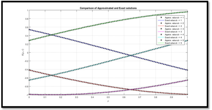
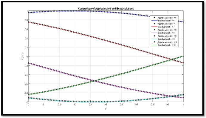
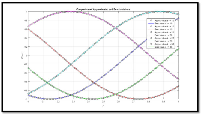
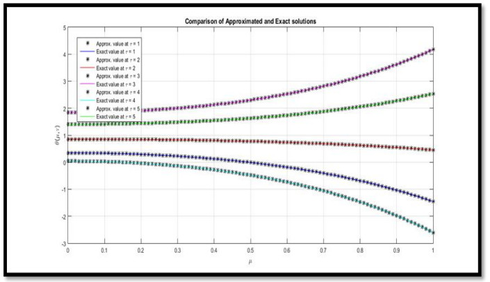
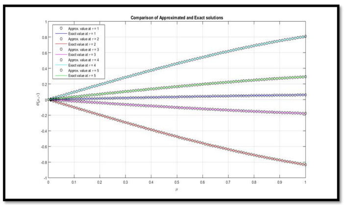
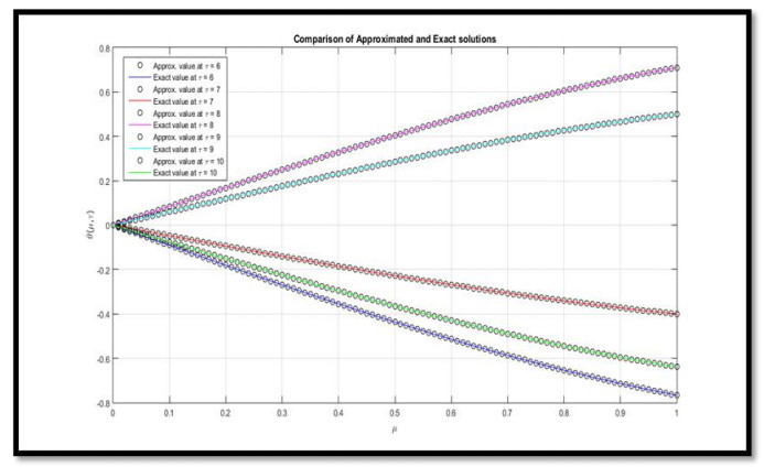
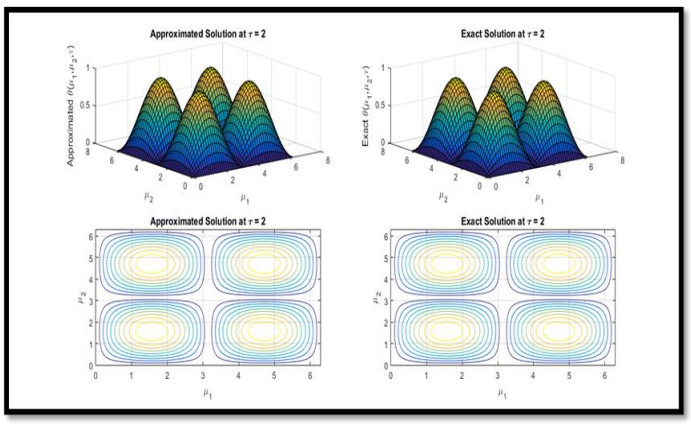
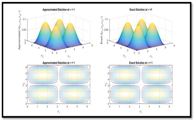
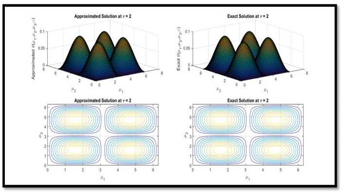
In the present section, the validity of the proposed regime is affirmed vias graphical and tabular analysis of the results. In , approx. and exact profiles are matched at $\tau$ = 1, 2, 3, 4, and 5 for Example 1. In , matching of approx. and exact profiles are provided at $\tau$ = 6, 7, 8, 9, and 10 for Example 1. A wide range of time levels is checked for compatibility. In , a match of approx. and exact profiles is provided at $\tau$ = 1.0, 1.5, 2.0, 2.5 and 3.0 for Example 2. is related to the approx. and exact profile compatibility at $\tau$ = 1, 2, 3, 4, and 5 for Example 3. In , compatibility of approx. and exact profiles are matched at $\tau$ = 1, 2, 3, 4, and 5 for Example 4. In , approx.-exact compatibility is mentioned at $\tau$ = 6, 7, 8, 9, and 10 for Example 4. and are related to the mesh-contour and surface-contour presentations at $\tau$ = 1 and $\tau$ = 2 respectively for Example 5. and are related to the mesh-contour and surface-contour presentations at $\tau$ = 1 and $\tau$ = 2, respectively for Example 6.

Figure 1. Approx. and exact profiles at

$t$ = 1, 2, 3, 4 and 5 regarding Example 1.

DownLoad: Full-Size Img PowerPoint

Figure 2. Approx. and exact profiles at

$t$ = 6, 7, 8, 9, and 10 where

$N$ = 101 regarding Example 1.

DownLoad: Full-Size Img PowerPoint

Figure 3. Approx. and exact profiles at

$t$ = 1.0, 1.5, 2.0, 2.5, and 3.0 where

$N$ = 101 regarding Example 2.

DownLoad: Full-Size Img PowerPoint

Figure 4. Approx. and exact profiles at

$t$ = 1, 2, 3, 4, and 5 where

$N$ = 101 regarding Example 3.

DownLoad: Full-Size Img PowerPoint

Figure 5. Approx. and exact profiles at

$t$ = 1, 2, 3, 4, and 5 where

$N$ = 101 regarding Example 4.

DownLoad: Full-Size Img PowerPoint

Figure 6. Approx. and exact profiles at

$t$ = 6, 7, 8, 9, and 10 where

$N$ = 101 regarding Example 4.

DownLoad: Full-Size Img PowerPoint

Figure 7. Approx. and exact profiles at

$t$ = 1 where

$N$ = 51 regarding Example 5.

DownLoad: Full-Size Img PowerPoint

Figure 8. Approx. and exact profiles at

$t$ = 2 where

$N$ = 51 regarding Example 5.

DownLoad: Full-Size Img PowerPoint

Figure 9. Approx. and exact profiles at

$t$ = 1, where

$N$ = 101,

$z$ = 0.1 regarding Example 6.

DownLoad: Full-Size Img PowerPoint

Figure 10. Approx. and exact profiles at

$t$ = 2 where

$N$ = 101,

$z$ = 0.1 regarding Example 6.

DownLoad: Full-Size Img PowerPoint

Via Tables 3–8, it can be affirmed that the approx. and exact profiles are matched for a wide range of time levels regarding the proposed scheme. Error analysis and convergence property are done by means of Tables 3–. In –, ${L}_{\infty }$ errors are provided at various grid points and time levels. Via –, it is reported that on increasing the number of grid points at different time levels, ${L}_{\infty }$ error got reduced, and in most of the cases, convergence is affirmed up to higher order.

6. Conclusions

In the present study, the motive is to deal with $1D$ , $2D$ , and $3D$ time-fractional Schr $\ddot{o}$ dinger equations regarding the approx.-analytical outcome. Shehu transform ADM is incorporated for this purpose. The prime key of a developed regime is it's easy-to-implement approach and accurate results. Furthermore, with the aid of the six mentioned examples, it is ensured that the retrieved approximated profiles are compatible with exact profiles. The graphical matching aspect between the approximated and exact results is also notified, which ensures that the developed technique is a good alternative to solve complex natured time-fractional PDEs. ${L}_{\infty }$ error is mentioned in–. Via mentioned tables, it is ensured that the proposed methodology is convergent, as on increasing the number of grid points, ${L}_{\infty }$ error got reduced. With the aid of the developed regime, various complex natured fractional PDEs can be easily solved.

Acknowledgments

This research received funding support from the NSRF via the Program Management Unit for Human Resources & Institutional Development, Research and Innovation (grant number B05F640092).

Conflict of interest

The authors declare no conflict of interest.

References

[1]	P. Diolez, V. Deschodt-Arsac, G. Raffard, C. Simon, P. D. Santos, E. Thiaudière, et al., Modular regulation analysis of heart contraction: application to in situ demonstration of a direct mitochondrial activation by calcium in beating heart, Am. J. Physiol.-Reg., I., 293 (2007), R13–R19.
[2]	M. Luo, M. E. Anderson, Mechanisms of altered Ca²⁺ handling in heart failure, Circ. Res., 113 (2013), 690–708.
[3]	A. Takeuchi, S. Matsuoka, Integration of mitochondrial energetics in heart with mathematical modelling, J. Physiol.-London, 598 (2020), 1443–1457.
[4]	G. Magnus, J. Keizer, Minimal model of $\beta$ -cell mitochondrial Ca $^{2+}$ handling, Am. J. Physiol.-Cell Ph., 273 (1997), C717–C733. doi: 10.1152/ajpcell.1997.273.2.C717
[5]	R. Bertram, M. G. Pedersen, D. S. Luciani, A. Sherman, A simplified model for mitochondrial ATP production, J. Theor. Biol., 243 (2006), 575–586. doi: 10.1016/j.jtbi.2006.07.019
[6]	C. C. Mitchell, D. G. Schaeffer, A two-current model for the dynamics of cardiac membrane, B. Math. Biol., 65 (2003), 767–793.
[7]	K. H. ten Tusscher, A. V. Panfilov, Alternans and spiral breakup in a human ventricular tissue model, Am. J. Physiol. Heart C., 291 (2006), H1088–1100.
[8]	T. L. Hill, Free energy transduction in biology: the steady-state kinetic and thermodynamic formalism, Academic Press, 1977.
[9]	D. Pietrobon, S. R. Caplan, Flow-force relationships for a six-state proton pump model: intrinsic uncoupling, kinetic equivalence of input and output forces, and domain of approximate linearity, Biochemistry-US, 24 (1985), 5764–5776. doi: 10.1021/bi00342a012
[10]	M.-H. T. Nguyen, M. S. Jafri, Mitochondrial calcium signaling and energy metabolism, Ann. N.Y. Acad. Sci., 1047 (2005), 127–137.
[11]	M.-H. T. Nguyen, S. J. Dudycha, M. S. Jafri, Effect of Ca²⁺ on cardiac mitochondrial energy production is modulated by Na⁺ and H⁺ dynamics, Am. J. Physiol.-Cell Ph., 292 (2007), C2004–C2020.
[12]	S. Cortassa, M. A. Aon, E. Marbân, R. L. Winslow, B. O'Rourke, An integrated model of cardiac mitochondrial energy metabolism and calcium dynamics, Biophys. J., 84 (2003), 2734–2755. doi: 10.1016/S0006-3495(03)75079-6
[13]	S. Cortassa, B. O'Rourke, R. L. Winslow, M. A. Aon, Control and regulation of mitochondrial energetics in an integrated model of cardiomyocyte function, Biophys. J., 96 (2009), 2466–2478.
[14]	L. D. Gauthier, J. L. Greenstein, S. Cortassa, B. O'Rourke, R. L. Winslow, A computational model of reactive oxygen species and redox balance in cardiac mitochondria, Biophys. J., 105 (2013), 1045–1056. doi: 10.1016/j.bpj.2013.07.006
[15]	G. Magnus, J. Keizer, Model of $\beta$ -cell mitochondrial calcium handling and electrical activity. I. Cytoplasmic variables, Am. J. Physiol.-Cell Ph., 274 (1998), C1158–C1173.
[16]	M. D. Brand, The stoichiometry of the exchange catalysed by the mitochondrial calcium/sodium antiporter, Biochem. J., 229 (1985), 161–166.
[17]	T. Matsuda, K. Takuma, A. Baba, Na⁺-Ca²⁺ exchanger: physiology and pharmacology, Jpn. J. Pharmacol., 74 (1997), 1–20.
[18]	T. E. Gunter, D. R. Pfeiffer, Mechanisms by which mitochondria transport calcium, Am. J. Physiol.-Cell Ph., 258 (1990), C755–C786.
[19]	D. E. Wingrove, T. Gunter, Kinetics of mitochondrial calcium transport. I. Characteristics of the sodium-independent calcium efflux mechanism of liver mitochondria, J. Biol. Chem., 261 (1986), 15159–15165. doi: 10.1016/S0021-9258(18)66846-2
[20]	G. C. Brown, The leaks and slips of bioenergetic membranes, FASEB J., 6 (1992), 2961–2965.
[21]	M. D. Brand, L.-F. Chien, P. Diolez, Experimental discrimination between proton leak and redox slip during mitochondrial electron transport, Biochem. J., 297 (Pt 1) (1994), 27–29.
[22]	G. Krishnamoorthy, P. C. Hinkle, Non-ohmic proton conductance of mitochondria and liposomes, Biochemistry-US, 23 (1984), 1640–1645.
[23]	C. Colin, Développement de nouvelles méthodes de microscopie et d'électrochimie pour des analyses multi-paramétriques de mitochondries individuelles cardiaques (in French), Theses, Université de Bordeaux, 2020, Available from: https://tel.archives-ouvertes.fr/tel-03116368.
[24]	Carlos M. Palmeira, António J. Moreno (eds.), Mitochondrial Bioenergetics, vol. 1782 of Methods in Molecular Biology, Humana Press, 2008.
[25]	B. Chance, W. G.R., Respiratory enzymes in oxidative phosphorylation: III. The steady state, J. Biol. Chem., 217 (1955), 409–427. doi: 10.1016/S0021-9258(19)57191-5
[26]	A. Saltelli, M. Ratto, T. Andres, F. Campolongo, J. Cariboni, D. Gatelli, et al., Global sensitivity analysis: the primer, John Wiley & Sons, 2008.
[27]	J. Herman, W. Usher, SALib: An open-source Python library for Sensitivity Analysis, J. Open Source Softw., 2 (2017), 97. doi: 10.21105/joss.00097
[28]	F. Wu, F. Yang, K. Vinnakota, D. Beard, Computer modeling of mitochondrial tricarboxylic acid cycle, oxidative phosphorylation, metabolite transport, and electrophysiology, J. Biol. Chem., 282 (2007), 24525–24537. doi: 10.1074/jbc.M701024200

mbe-18-05-291-s001.zip

This article has been cited by:

1.	Nourhane Attia, Ali Akgül, Djamila Seba, Abdelkader Nour, Manuel De la Sen, Mustafa Bayram, An Efficient Approach for Solving Differential Equations in the Frame of a New Fractional Derivative Operator, 2023, 15, 2073-8994, 144, 10.3390/sym15010144
2.	Mamta Kapoor, Samanyu Khosla, Series Solution to Fractional Telegraph Equations Using an Iterative Scheme Based on Yang Transform, 2024, 0971-3514, 10.1007/s12591-024-00679-w
3.	Mamta Kapoor, Varun Joshi, A comparative study of Sumudu HPM and Elzaki HPM for coupled Burgers’ equation, 2023, 9, 24058440, e15726, 10.1016/j.heliyon.2023.e15726
4.	M. L. Rupa, K. Aruna, Optical solitons of time fractional Kundu–Eckhaus equation and massive Thirring system arises in quantum field theory, 2024, 56, 0306-8919, 10.1007/s11082-023-05914-2

Reader Comments

Your name:*

Email:*
© 2021 the Author(s), licensee AIMS Press. This is an open access article distributed under the terms of the Creative Commons Attribution License (http://creativecommons.org/licenses/by/4.0)