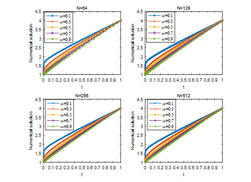
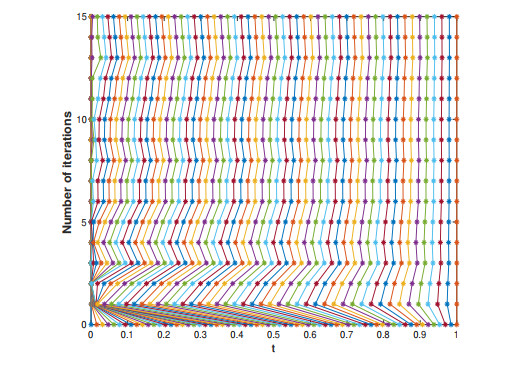
A nonlinear initial value problem whose differential operator is a Caputo derivative of order $ \alpha $ with $ 0 < \alpha < 1 $ is studied. By using the Riemann-Liouville fractional integral transformation, this problem is reformulated as a Volterra integral equation, which is discretized by using the right rectangle formula. Both a priori and an a posteriori error analysis are conducted. Based on the a priori error bound and mesh equidistribution principle, we show that there exists a nonuniform grid that gives first-order convergent result, which is robust with respect to $ \alpha $. Then an a posteriori error estimation is derived and used to design an adaptive grid generation algorithm. Numerical results complement the theoretical findings.
Citation: Yong Zhang, Xiaobing Bao, Li-Bin Liu, Zhifang Liang. Analysis of a finite difference scheme for a nonlinear Caputo fractional differential equation on an adaptive grid[J]. AIMS Mathematics, 2021, 6(8): 8611-8624. doi: 10.3934/math.2021500
A nonlinear initial value problem whose differential operator is a Caputo derivative of order $ \alpha $ with $ 0 < \alpha < 1 $ is studied. By using the Riemann-Liouville fractional integral transformation, this problem is reformulated as a Volterra integral equation, which is discretized by using the right rectangle formula. Both a priori and an a posteriori error analysis are conducted. Based on the a priori error bound and mesh equidistribution principle, we show that there exists a nonuniform grid that gives first-order convergent result, which is robust with respect to $ \alpha $. Then an a posteriori error estimation is derived and used to design an adaptive grid generation algorithm. Numerical results complement the theoretical findings.

| [1] | R. Magin, Fractional Calculus in Bioengineering, Begell House Publishers, Redding, 2006. |
| [2] | A. Kaur, P. S. Takhar, D. M. Smith, J. E. Mann, M. M. Brashears, Fractional differential equations based modeling of microbial survival and growth curves: Model development and experimental validation, Food Eng. Phy. Properties, 73 (2008), 403-414. |
| [3] | D. Lokenath, Recent applications of fractional calculus to science and engineering, Int. J. Math. Math. Sci., 54 (2003), 3413-3442. |
| [4] |
P. A. Naik, J. Zu, K. M. Owolabi, Modeling the mechanics of viral kinetics under immune control during primary infection of HIV-1 with treatment in fractional order, Physica A., 545 (2020), 123816. doi: 10.1016/j.physa.2019.123816

|
| [5] |
P. A. Naik, J. Zu, K. M. Owolabi, Global dynamics of a fractional order model for the transmission of HIV epidemic with optimal control, Chaos. Solition. Fract., 138 (2020), 109826. doi: 10.1016/j.chaos.2020.109826
|
| [6] |
P. A. Naik, K. M. Owolabi, M. Yavuz, Z. Jian, Chaotic dynamics of a fractional order HIV-1 model involving AIDS-related cancer cells, Chaos. Solition. Fract., 140 (2020), 110272 doi: 10.1016/j.chaos.2020.110272
|
| [7] |
K. M. Owolabi, B. Karaagac, Dynamics of multi-puls splitting process in one-dimensional Gray-Scott system with fractional order operator, Chaos. Soliton. Fract., 136 (2020), 109835. doi: 10.1016/j.chaos.2020.109835
|
| [8] |
C. Li, F. Zeng, The finite difference methods for fractional ordinary differential equations, Numer. Funct. Anal. Optim., 34 (2013), 149-179. doi: 10.1080/01630563.2012.706673
|
| [9] |
M. Stynes, J. L. Gracia, A finite difference method for a two-point boundary value problem with a Caputo fractional derivative, IMA J. Numer. Anal., 35 (2015), 698-721. doi: 10.1093/imanum/dru011
|
| [10] |
S. Vong, P. Lyu, X. Chen, S.-L. Lei, High order finite difference method for time-space fractional differential equations with Caputo and Riemann-Liouville derivatives, Numer. Algorithm., 72 (2016), 195-210. doi: 10.1007/s11075-015-0041-3
|
| [11] | K. M. Owolabi, Numerical simulation of fractional-order reaction-diffusion equations with the Riesz and Caputo derivatives, Neural. Comput. Appl., 2019. Available from: https://doi.org/10.1007/s00521-019-04350-2. |
| [12] | K. Nedaiasl, R. Dehbozorgi, Galerkin finite element method for nonlinear fractional differential equations, Numer. Algorithms., 2021. Available from: https://doi.org/10.1007/s11075-020-01032-2. |
| [13] |
H. Liang, M. Stynes, Collocation methods for general Caputo two-point boundary value problems, J. Sci. Comput., 76 (2018), 390-425. doi: 10.1007/s10915-017-0622-5
|
| [14] |
H. Liang, M. Stynes, Collocation methods for general Riemann-Liouville two-point boundary value problems, Adv. Comput. Math., 45 (2019), 897-928. doi: 10.1007/s10444-018-9645-1
|
| [15] |
N. Kopteva, M. Stynes, An efficient collocation method for a Caputo two-point boundary value problem, BIT Numer. Math., 55 (2015), 1105-1123. doi: 10.1007/s10543-014-0539-4
|
| [16] |
C. Wang, Z. Wang, L. Wang, A spectral collocation method for nonlinear fractional boundary value problems with a Caputo derivative, J. Sci. Comput., 76 (2018), 166-188. doi: 10.1007/s10915-017-0616-3
|
| [17] |
Z. Gu, Spectral collocation method for nonlinear Caputo fractional differential system, Adv. Comput. Math., 46 (2020), 66. doi: 10.1007/s10444-020-09808-9
|
| [18] |
M. Stynes, J. L. Gracia, A finite difference method for a two-point boundary value problem with a Caputo fractional derivative, IMA J. Numer. Anal., 35 (2015), 698-721. doi: 10.1093/imanum/dru011
|
| [19] |
J. Gracia, M. Stynes, Central difference approximation of convection in Caputo fractional derivative two-point boundary value problems, J. Comput. Appl. Math., 273 (2015), 103-115. doi: 10.1016/j.cam.2014.05.025
|
| [20] |
M. Stynes, E. O'Riordan, J. L. Gracia, Error analysis of a finite difference method on graded meshes for a time-fractional diffusion equation, SIAM J. Numer. Anal., 55 (2017), 1057-1079. doi: 10.1137/16M1082329
|
| [21] |
H. Liao, W. Mclean, J. Zhang, A discrete Grönwall inequality with applications to numerical scheme for sudiffusion problems, SIAM J. Numer. Anal., 57 (2019), 218-237. doi: 10.1137/16M1175742
|
| [22] |
J. L. Gracia, E. O'Riordan, M. Stynes, A fitted scheme for a Caputo initial-boundary value problem, J. Sci. Comput., 76 (2018), 583-609. doi: 10.1007/s10915-017-0631-4
|
| [23] | N. Kopteva, X. Meng, Error analysis for a fractional-derivative parabolic problem on quasi-graded meshes using barrier function, SIAM J. Numer. Anal., 2020, 58 (2020), 1217-1238. |
| [24] |
Z. Cen, L. B. Liu, J. Huang, A posteriori error estimation in maximum norm for a two-point boundary value problem with a Riemann-Liouville fractional derivative, Appl. Math. Lett., 102 (2020), 106086. doi: 10.1016/j.aml.2019.106086
|
| [25] |
L. B. Liu, Z. Liang, G. Long, Y. Liang, Convergence analysis of a finite difference scheme for a Riemann-Liouville fractional derivative two-point boundary value problem on an adaptive grid, J. Comput. Appl. Math., 375 (2020), 112809. doi: 10.1016/j.cam.2020.112809
|
| [26] |
J. Huang, Z. Cen, L. B. Liu, J. Zhao, An efficient numerical method for a Riemann-Liouville two-point boundary value problem, Appl. Math. Lett., 103 (2020), 106201. doi: 10.1016/j.aml.2019.106201
|
| [27] | Z. Cen, A. Le, A. Xu, A posteriori error analysis for a fractional differential equation, Int. J. Comput. Math., 94 (2017), 1182-1195. |
| [28] | L. B. Liu, Y. Chen, A posteriori error estimation and adaptive strategy for a nonlinear fractional differential equation, Int. J. Comput. Math., 2021. Available from: https://doi.org/10.1080/00207160.2021.1906420. |
| [29] | K. Diethelm, The analysis of fractional differential equations. Springer, Berlin, 2010. |
| [30] |
C. Li, Q. Yi, A. Chen, Finite difference methods with non-uniform meshes for nonlinear differential equations, J. Comput. Phys., 316 (2016), 614-631. doi: 10.1016/j.jcp.2016.04.039
|
| [31] |
H. Ye, J. Gao, Y. Ding, A generalized Grönwall inequality and its application to a fractional differential equation, J. Math. Anal. Appl., 328 (2007), 1075-1081. doi: 10.1016/j.jmaa.2006.05.061
|
Figures(2) / Tables(3)

Yong Zhang, Xiaobing Bao, Li-Bin Liu, Zhifang Liang. Analysis of a finite difference scheme for a nonlinear Caputo fractional differential equation on an adaptive grid[J]. AIMS Mathematics, 2021, 6(8): 8611-8624. doi: 10.3934/math.2021500


 DownLoad: