The COVID-19 pandemic has impacted communities differentially, with poorer and minority populations being more adversely affected. Prior rural health research suggests such disparities may be exacerbated during the pandemic and in remote parts of the U.S.
To understand the spread and impact of COVID-19 across the U.S., county level data for confirmed cases of COVID-19 were examined by Area Deprivation Index (ADI) and Metropolitan vs. Nonmetropolitan designations from the National Center for Health Statistics (NCHS). These designations were the basis for making comparisons between Urban and Rural jurisdictions.
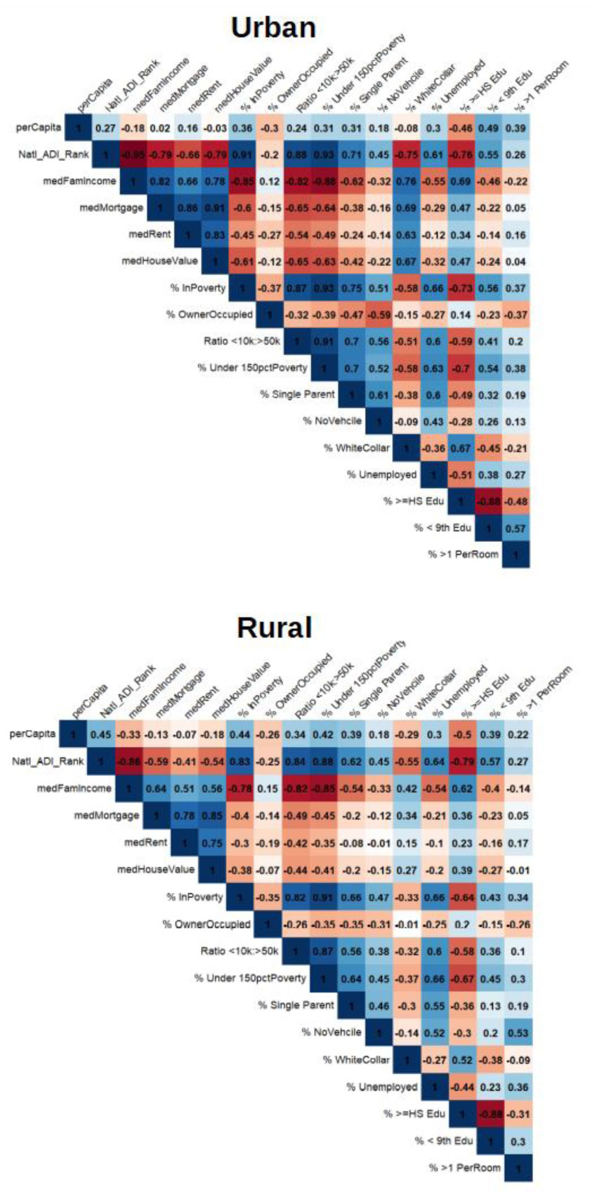
Kendall's Tau-B was used to compare effect sizes between jurisdictions on select ADI composites and well researched social determinants of health (SDH). Spearman coefficients and stratified Poisson modeling was used to explore the association between ADI and COVID-19 prevalence in the context of county designation.
Results show that the relationship between area deprivation and COVID-19 prevalence was positive and higher for rural counties, when compared to urban ones. Family income, property value and educational attainment were among the ADI component measures most correlated with prevalence, but this too differed between county type.
Though most Americans live in Metropolitan Areas, rural communities were found to be associated with a stronger relationship between deprivation and COVID-19 prevalence. Models predicting COVID-19 prevalence by ADI and county type reinforced this observation and may inform health policy decisions.
Citation: Christopher Kitchen, Elham Hatef, Hsien Yen Chang, Jonathan P Weiner, Hadi Kharrazi. Assessing the association between area deprivation index on COVID-19 prevalence: a contrast between rural and urban U.S. jurisdictions[J]. AIMS Public Health, 2021, 8(3): 519-530. doi: 10.3934/publichealth.2021042
The COVID-19 pandemic has impacted communities differentially, with poorer and minority populations being more adversely affected. Prior rural health research suggests such disparities may be exacerbated during the pandemic and in remote parts of the U.S.
To understand the spread and impact of COVID-19 across the U.S., county level data for confirmed cases of COVID-19 were examined by Area Deprivation Index (ADI) and Metropolitan vs. Nonmetropolitan designations from the National Center for Health Statistics (NCHS). These designations were the basis for making comparisons between Urban and Rural jurisdictions.
Kendall's Tau-B was used to compare effect sizes between jurisdictions on select ADI composites and well researched social determinants of health (SDH). Spearman coefficients and stratified Poisson modeling was used to explore the association between ADI and COVID-19 prevalence in the context of county designation.
Results show that the relationship between area deprivation and COVID-19 prevalence was positive and higher for rural counties, when compared to urban ones. Family income, property value and educational attainment were among the ADI component measures most correlated with prevalence, but this too differed between county type.
Though most Americans live in Metropolitan Areas, rural communities were found to be associated with a stronger relationship between deprivation and COVID-19 prevalence. Models predicting COVID-19 prevalence by ADI and county type reinforced this observation and may inform health policy decisions.

| [1] |
Yancy CW (2020) COVID-19 and African Americans. JAMA 323: 1891-1892. doi: 10.1001/jama.2020.6548

|
| [2] |
Laurencin CT, McClinton A (2020) The COVID-19 Pandemic: A Call to Action to Identify and Address Racial and Ethnic Disparities. J Racial Ethn Health Disparities 7: 398-402. doi: 10.1007/s40615-020-00756-0
|
| [3] | Centers for Disease Control and Prevention Health, United States Spotlight. Racial and Ethnic Disparities in Health Disease (2019) .Available from: https://www.cdc.gov/nchs/hus/spotlight/HeartDiseaseSpotlight_2019_0404.pdf. |
| [4] |
Upshaw TL, Brown C, Smith R, et al. (2021) Social determinants of COVID-19 incidence and outcomes: A rapid review. PLOS One 16. doi: 10.1371/journal.pone.0248336
|
| [5] |
Mueller JT, McConnell K, Burow PB, et al. (2021) Impacts of the COVID-19 pandemic on rural America. P Natl Acad Sci 118. doi: 10.1073/pnas.2019378118
|
| [6] |
Rajib P, Arif AA, Adeyemi O, et al. (2020) Progression of COVID-19 From Urban to Rural Areas in the United States: A Spatiotemporal Analysis of Prevalence Rates. J Rural Health 36: 591-601. doi: 10.1111/jrh.12486
|
| [7] |
Peters DJ (2020) Community Susceptibility and Resiliency to COVID-19 Across the Rural-Urban Continuum in the United States. J Rural Health 36: 446-456. doi: 10.1111/jrh.12477
|
| [8] |
Zhang CH, Schwartz GG (2020) Spatial Disparities in Coronavirus Incidence and Mortality in the United States: An Ecological Analysis as of May 2020. J Rural Health 36: 433-445. doi: 10.1111/jrh.12476
|
| [9] |
James CV, Moonesinghe R, Wilson-Frederick SM, et al. (2017) Racial/Ethnic Health Disparities Among Rural Adults-United States, 2012–2015. MMWR Surveill Summ 66: 1-9. doi: 10.15585/mmwr.ss6623a1
|
| [10] |
Hartley D (2004) Rural Health Disparities, Population Health, and Rural Culture. Am J Public Health 94: 1675-1678. doi: 10.2105/AJPH.94.10.1675
|
| [11] |
Ranscombe P (2020) Rural areas at risk during COVID-19 pandemic. Lancet Infect Dis Lancet Infect Dis 20: 545. doi: 10.1016/S1473-3099(20)30301-7
|
| [12] |
Erwin C, Aultman J, Harter T, et al. (2020) Rural and Remote Communities: Unique Ethical Issues in the COVID-19 Pandemic. Am J Bioeth 20: 117-120. doi: 10.1080/15265161.2020.1764139
|
| [13] |
Singh GK (2003) Area deprivation and widening inequalities in US mortality, 1969–1998. Am J Public Health 93: 1137-1143. doi: 10.2105/AJPH.93.7.1137
|
| [14] | Knighton AJ, Savitz L, Belnap T, et al. (2016) Introduction of an Area Deprivation Index Measuring Patient Socioeconomic Status in an Integrated Health System: Implications for Population Health. EGEMS (Wash DC) 4: 1238. |
| [15] |
Hatef E, Chang HY, Kitchen C, et al. (2020) Assessing the impact of neighborhood socioeconomic characteristics on COVID-19 prevalence across seven states in the United States. Front Public Health 8: 571808. doi: 10.3389/fpubh.2020.571808
|
| [16] | Oral E, Straif-Bourgeois S, Rung AL, et al. (2020) The effect of area deprivation on COVID-19 risk in Louisiana. PLOS One 72: 1-12. |
| [17] |
Hendricks B, Paul R, Smith C, et al. (2021) Coronavirus testing disparities associated with community level deprivation, racial inequalities, and food insecurity in West Virginia. Ann Epidemiol 59: 44-49. doi: 10.1016/j.annepidem.2021.03.009
|
| [18] | Flanagan BE, Gregory EW, Hallisey EJ, et al. (2011) A Social Vulnerability Index for Disaster Management. J Home Secur Emerg Manag 8: 1-24. |
| [19] | Kharrazi H, Gudzune K, Weiner JP (2020) A population health segmentation framework for balancing medical need and COVID-19 risk during and after the pandemic. Health Affairs Blog Available from: https://www.healthaffairs.org/do/10.1377/hblog20200902.328533/full/. |
| [20] |
Dong E, Du H, Gardner L (2020) An interactive web-based dashboard to track COVID-19 in real time. Lancet Infect Dis 20: 533-534. doi: 10.1016/S1473-3099(20)30120-1
|
| [21] | Dong E, Du H, Gardner L (2020) COVID-19 Data Repository by the Center for Systems Science and Engineering (CSSE) at Johns Hopkins University Baltimore, MD: GitHub; Date last modified June 9, 2020, Available from: https://github.com/CSSEGISandData/COVID-19. |
| [22] | Chin T, Kahn R, Li R, et al. (2020) U.S. county-level characteristics to inform equitable COVID-19 response. medRxiv . |
| [23] | Fauver JR, Petrone ME, Hodcroft EB, et al. (2020) Coast-to-coast spread of SARS-CoV-2 in the United States revealed by genomic epidemiology. medRxiv . |
| [24] | Yuan X, Xu J, Hussain S, et al. (2020) Trends and prediction in daily incidence and deaths of COVID-19 in the United States: a search-interest based model. Preprint. medRxiv . |
| [25] | Kaiser Family Foundation Population Distribution by Race/Ethnicity Available from: https://www.kff.org/other/state-indicator/distribution-by-raceethnicity/?currentTimeframe=0&sortModel=%7B%22coIId%22:%22Location%22.%22sort%22:%22asc%22%7D. |
| [26] | The United States Census Bureau American community survey (ACS) Available from: https://www.census.gov/programs-surveys/acs/. |
| [27] |
Kind AJH, Jencks S, Brock J, et al. (2014) Neighborhood socioeconomic disadvantage and 30-day rehospitalizations: an analysis of Medicare data. Ann Intern Med 161: 765-774. doi: 10.7326/M13-2946
|
| [28] |
Figueroa JF, Frakt AB, Jha AK (2020) Addressing Social Determinants of Health: Time for a Polysocial Risk Score. JAMA 323: 1553-1554. doi: 10.1001/jama.2020.2436
|
| [29] | Ingram DD, Franco SJ (2014) 2013 NCHS urban-rural classification scheme for counties. Vital Health Stat 2: Available from: https://www.cdc.gov/nchs/data/series/sr_02/sr02_166.pdf. |
| [30] | Centers for Disease Control and Prevention National Center for Health Statistics: NCHS Urban-Rural Classification Scheme for Counties (2020) .Available from: https://www.cdc.gov/nchs/data_access/urban_rural.htm. |
| [31] |
Faraway J (2005) Extending the Linear Model with R (Texts in Statistical Science) Chapman & Hall/CRC. doi: 10.1201/b15416
|
| [32] |
Heinzl H, Mittleböck M (2003) Pseudo R-squared measures for Poisson regression models with over- or underdispersion. Comput Stat Data An 44: 253-271. doi: 10.1016/S0167-9473(03)00062-8
|
| [33] |
Cuadros DF, Branscum AJ, Mukandavire Z, et al. (2021) Dynamics of the COVID-19 epidemic in urban and rural areas in the United States. Ann Epidemiol 59: 16-20. doi: 10.1016/j.annepidem.2021.04.007
|
| [34] | Guha A, Bonsu J, Dey A, et al. (2020) Community and Socioeconomic Factors Associated with COVID-19 in the United States: Zip code level cross sectional analysis. medRxiv . |
| [35] |
Zhang X, Hailu B, Tabor D, et al. (2019) Role of Health Information Technology in Addressing health Disparities. Medical Care 57: S115-S120. doi: 10.1097/MLR.0000000000001092
|
| [36] |
Park J, Erikson C, Han X, et al. (2018) Are State Telehealth Policies Associated With The Use Of Telehealth Services Among Underserved Populations? Health Aff (Millwood) 37: 2060-2068. doi: 10.1377/hlthaff.2018.05101
|
| [37] |
Krakow M, Hesse B, Oh A, et al. (2019) Addressing Rural Geographic Disparities Through Health IT Initial Findings From the Health Information National Trends Survey. Medical Care 57: S127-S132. doi: 10.1097/MLR.0000000000001028
|
| [38] |
Hatef E, Kitchen C, Chang HY, et al. (2020) Early relaxation of community mitigation policies and risk of COVID-19 resurgence in the United States. Prev Med 145: 106435. doi: 10.1016/j.ypmed.2021.106435
|

Figures(2) / Tables(3)

Christopher Kitchen, Elham Hatef, Hsien Yen Chang, Jonathan P Weiner, Hadi Kharrazi. Assessing the association between area deprivation index on COVID-19 prevalence: a contrast between rural and urban U.S. jurisdictions[J]. AIMS Public Health, 2021, 8(3): 519-530. doi: 10.3934/publichealth.2021042


 DownLoad: