A machine learning approach to enhance the SUPG stabilization method for advection-dominated differential problems

1.
Oliver Wyman Srl, Via Broletto 16, 20121, Milano, Italy
2.
MOX, Laboratory of Scientific Computing, Dipartimento di Matematica, Politecnico di Milano, Piazza Leonardo da Vinci, 32, 20133, Milano, Italy

Received: 30 October 2021 Revised: 23 March 2022 Accepted: 21 April 2022 Published: 12 May 2022

We propose using machine learning and artificial neural networks (ANNs) to enhance residual-based stabilization methods for advection-dominated differential problems. Specifically, in the context of the finite element method, we consider the streamline upwind Petrov-Galerkin (SUPG) stabilization method and we employ ANNs to optimally choose the stabilization parameter on which the method relies. We generate our dataset by solving optimization problems to find the optimal stabilization parameters that minimize the distances among the numerical and the exact solutions for different data of differential problem and the numerical settings of the finite element method, e.g., mesh size and polynomial degree. The dataset generated is used to train the ANN, and we used the latter "online" to predict the optimal stabilization parameter to be used in the SUPG method for any given numerical setting and problem data. We show, by means of 1D and 2D numerical tests for the advection-dominated differential problem, that our ANN approach yields more accurate solution than using the conventional stabilization parameter for the SUPG method.
- partial differential equations,
- finite element method,
- stabilization methods,
- streamline upwind Petrov-Galerkin,
- machine learning,
- artificial neural networks
Citation: Tommaso Tassi, Alberto Zingaro, Luca Dede'. A machine learning approach to enhance the SUPG stabilization method for advection-dominated differential problems[J]. Mathematics in Engineering, 2023, 5(2): 1-26. doi: 10.3934/mine.2023032

Related Papers:

Abstract

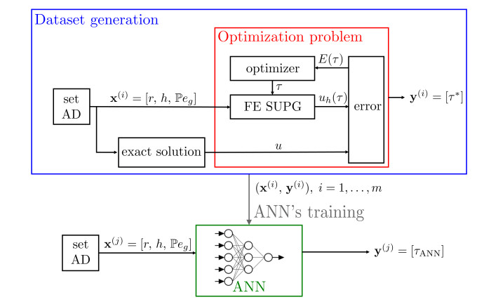
We propose using machine learning and artificial neural networks (ANNs) to enhance residual-based stabilization methods for advection-dominated differential problems. Specifically, in the context of the finite element method, we consider the streamline upwind Petrov-Galerkin (SUPG) stabilization method and we employ ANNs to optimally choose the stabilization parameter on which the method relies. We generate our dataset by solving optimization problems to find the optimal stabilization parameters that minimize the distances among the numerical and the exact solutions for different data of differential problem and the numerical settings of the finite element method, e.g., mesh size and polynomial degree. The dataset generated is used to train the ANN, and we used the latter "online" to predict the optimal stabilization parameter to be used in the SUPG method for any given numerical setting and problem data. We show, by means of 1D and 2D numerical tests for the advection-dominated differential problem, that our ANN approach yields more accurate solution than using the conventional stabilization parameter for the SUPG method.

References

[1]	M. Abadi, A. Agarwal, P. Barham, E. Brevdo, Z. Chen, C. Citro. et al., TensorFlow: Large-scale machine learning on heterogeneous systems, arXiv: 1603.04467.
[2]	M. S. Alnæs, J. Blechta, J. Hake, A. Johansson, B. Kehlet, A. Logg, et al., The fenics project version 1.5, Archive of Numerical Software, 3 (2015), 9–23. https://doi.org/10.11588/ans.2015.100.20553 doi: 10.11588/ans.2015.100.20553
[3]	Y. Bazilevs, V. M. Calo, J. A. Cottrell, T. J. R. Hughes, A. Reali, G. Scovazzi, Variational multiscale residual-based turbulence modeling for large eddy simulation of incompressible flows, Comput. Method. Appl. Mech. Eng., 197 (2007), 173–201. https://doi.org/10.1016/j.cma.2007.07.016 doi: 10.1016/j.cma.2007.07.016
[4]	N. Bénard, J. Pons-Prats, J. Périaux, G. Bugeda, P. Braud, J. P. Bonnet, et al., Turbulent separated shear flow control by surface plasma actuator: experimental optimization by genetic algorithm approach, Exp. Fluids, 57 (2016), 22. https://doi.org/10.1007/s00348-015-2107-3 doi: 10.1007/s00348-015-2107-3
[5]	P. B. Bochev, C. R. Dohrmann, M. D. Gunzburger, Stabilization of low-order mixed finite elements for the Stokes equations, SIAM J. Numer. Anal., 44 (2016), 82–101. https://doi.org/10.1137/S0036142905444482 doi: 10.1137/S0036142905444482
[6]	A. N. Brooks, T. J. R. Hughes, Streamline upwind/Petrov-Galerkin formulations for convection dominated flows with particular emphasis on the incompressible Navier-Stokes equations, Comput. Method. Appl. Mech. Eng., 32 (1982), 199–259. https://doi.org/10.1016/0045-7825(82)90071-8 doi: 10.1016/0045-7825(82)90071-8
[7]	C. Canuto, M. Y. Hussaini, A. Quarteroni, T. A. Zang, Spectral methods. Fundamentals in single domains, Berlin, Heidelberg: Springer, 2006.
[8]	R. Codina, On stabilized finite element methods for linear systems of convection-diffusion-reaction equations, Comput. Method. Appl. Mech. Eng., 188 (2000), 61–82. https://doi.org/10.1016/S0045-7825(00)00177-8 doi: 10.1016/S0045-7825(00)00177-8
[9]	R. Codina, Analysis of a stabilized finite element approximation of the Oseen equations using orthogonal subscales, Appl. Numer. Math., 58 (2008), 264–283. https://doi.org/10.1016/j.apnum.2006.11.011 doi: 10.1016/j.apnum.2006.11.011
[10]	R. Codina, J. Principe, O. Guasch, S. Badia, Time dependent subscales in the stabilized finite element approximation of incompressible flow problems, Comput. Method. Appl. Mech. Eng., 196 (2007), 2413–2430. https://doi.org/10.1016/j.cma.2007.01.002 doi: 10.1016/j.cma.2007.01.002
[11]	B. Colvert, M. Alsalman, E. Kanso, Classifying vortex wakes using neural networks, Bioinspir. Biomim., 13 (2018), 025003. https://doi.org/10.1088/1748-3190/aaa787 doi: 10.1088/1748-3190/aaa787
[12]	J. A. Cottrell, T. J. R. Hughes, Y. Bazilevs, Isogeometric analysis: Toward integration of CAD and FEA, John Wiley & Sons, 2009. https://doi.org/10.1002/9780470749081
[13]	N. Discacciati, J. S. Hesthaven, D. Ray, Controlling oscillations in high-order discontinuous Galerkin schemes using artificial viscosity tuned by neural networks, J. Comput. Phys., 409 (2020), 109304. https://doi.org/10.1016/j.jcp.2020.109304 doi: 10.1016/j.jcp.2020.109304
[14]	K. Duraisamy, G. Iaccarino, H. Xiao, Turbulence modeling in the age of data, Annu. Rev. Fluid Mech., 51 (2019), 357–377. https://doi.org/10.1146/annurev-fluid-010518-040547 doi: 10.1146/annurev-fluid-010518-040547
[15]	D. Forti, L. Dede', Semi-implicit BDF time discretization of the Navier–Stokes equations with VMS-LES modeling in a high performance computing framework, Comput. Fluids, 117 (2015), 168–182. https://doi.org/10.1016/j.compfluid.2015.05.011 doi: 10.1016/j.compfluid.2015.05.011
[16]	L. P. Franca, S. L. Frey, T. J. R. Hughes, Stabilized finite element methods: I. application to the advective-diffusive model, Comput. Method. Appl. Mech. Eng., 95 (1992), 253–276. https://doi.org/10.1016/0045-7825(92)90143-8 doi: 10.1016/0045-7825(92)90143-8
[17]	S. Fresca, L. Dede', A. Manzoni, A comprehensive deep learning-based approach to reduced order modeling of nonlinear time-dependent parametrized PDEs, J. Sci. Comput., 87 (2021), 61. https://doi.org/10.1007/s10915-021-01462-7 doi: 10.1007/s10915-021-01462-7
[18]	A. C. Galeao, R. C. Almeida, S. M. C. Malta, A. F. D. Loula, Finite element analysis of convection dominated reaction–diffusion problems, Appl. Numer. Math., 48 (2004), 205–222. https://doi.org/10.1016/j.apnum.2003.10.002 doi: 10.1016/j.apnum.2003.10.002
[19]	I. Goodfellow, Y. Bengio, A. Courville, Deep learning, MIT Press, 2016.
[20]	M. Guo, J. S. Hesthaven, Data-driven reduced order modeling for time-dependent problems, Comput. Method. Appl. Mech. Eng., 345 (2019), 75–99. https://doi.org/10.1016/j.cma.2018.10.029 doi: 10.1016/j.cma.2018.10.029
[21]	J. S. Hesthaven, S. Ubbiali, Non-intrusive reduced order modeling of nonlinear problems using neural networks, J. Comput. Phys., 363 (2018), 55–78. https://doi.org/10.1016/j.jcp.2018.02.037 doi: 10.1016/j.jcp.2018.02.037
[22]	T. J. R. Hughes, The finite element method: linear static and dynamic finite element analysis, Courier Corporation, 2012.
[23]	M. Janssens, S. J. Hulshoff, Advancing artificial neural network parameterisation for atmospheric turbulence using a variational multiscale model, J. Adv. Model. Earth Syst., 14 (2022), e2021MS002490. https://doi.org/10.1029/2021MS002490 doi: 10.1029/2021MS002490
[24]	M. Janssens, Machine learning of atmospheric turbulence in a variational multiscale model, 2019. Available from: http://resolver.tudelft.nl/uuid:bd090309-305e-4c04-93b7-64f1b79df8d4.
[25]	V. John, P. Knobloch, On spurious oscillations at layers diminishing (sold) methods for convection–diffusion equations: Part I–A review, Comput. Method. Appl. Mech. Eng., 196 (2007), 2197–2215. https://doi.org/10.1016/j.cma.2006.11.013 doi: 10.1016/j.cma.2006.11.013
[26]	Keras. Available from: https://keras.io.
[27]	G. Kutyniok, P. Petersen, M. Raslan, R. Schneider, A theoretical analysis of deep neural networks and parametric PDEs, Constr. Approx., 55 (2021), 73–125. https://doi.org/10.1007/s00365-021-09551-4 doi: 10.1007/s00365-021-09551-4
[28]	M. Milano, P. Koumoutsakos, Neural network modeling for near wall turbulent flow, J. Comput. Phys., 182 (2002), 1–26. https://doi.org/10.1006/jcph.2002.7146 doi: 10.1006/jcph.2002.7146
[29]	S. Mishra, A machine learning framework for data driven acceleration of computations of differential equations, Mathematics in Engineering, 1 (2019), 118–146. https://doi.org/10.3934/Mine.2018.1.118 doi: 10.3934/Mine.2018.1.118
[30]	T. M. Mitchell, Machine learning, New York: McGraw-hill, 1997.
[31]	P. Neittaanmaki, S. Repin, Artificial intelligence and computational science, In: Computational sciences and artificial intelligence in industry, 76 (2022), 27–35. https://doi.org/10.1007/978-3-030-70787-3_3
[32]	G. Novati, L. Mahadevan, P. Koumoutsakos, Controlled gliding and perching through deep-reinforcement-learning, Phys. Rev. Fluids, 4 (2019), 093902. https://doi.org/10.1103/PhysRevFluids.4.093902 doi: 10.1103/PhysRevFluids.4.093902
[33]	A. Quarteroni, A. Valli, Numerical approximation of partial differential equations, Berlin, Heidelberg: Springer, 1994. https://doi.org/10.1007/978-3-540-85268-1
[34]	A. Quarteroni, Numerical models for differential problems, 3 Eds., Cham: Springer, 2017. https://doi.org/10.1007/978-3-319-49316-9
[35]	M. Raissi, G. E. Karniadakis, Hidden physics models: Machine learning of nonlinear partial differential equations, J. Comput. Phys., 357 (2018), 125–141. https://doi.org/10.1016/j.jcp.2017.11.039 doi: 10.1016/j.jcp.2017.11.039
[36]	M. Raissi, P. Perdikaris, G. E. Karniadakis, Machine learning of linear differential equations using Gaussian processes, J. Comput. Phys., 348 (2017), 683–693. https://doi.org/10.1016/j.jcp.2017.07.050 doi: 10.1016/j.jcp.2017.07.050
[37]	M. Raissi, P. Perdikaris, G. E. Karniadakis, Physics-informed neural networks: A deep learning framework for solving forward and inverse problems involving nonlinear partial differential equations, J. Comput. Phys., 378 (2019), 686–707. https://doi.org/10.1016/j.jcp.2018.10.045 doi: 10.1016/j.jcp.2018.10.045
[38]	T. C. Rebollo, B. M. Dia, A variational multi-scale method with spectral approximation of the sub-scales: Application to the 1D advection–diffusion equations, Comput. Method. Appl. Mech. Eng., 285 (2015), 406–426. https://doi.org/10.1016/j.cma.2014.11.025 doi: 10.1016/j.cma.2014.11.025
[39]	F. Regazzoni, L. Dede', A. Quarteroni, Machine learning of multiscale active force generation models for the efficient simulation of cardiac electromechanics, Comput. Method. Appl. Mech. Eng., 370 (2020), 113268. https://doi.org/10.1016/j.cma.2020.113268 doi: 10.1016/j.cma.2020.113268
[40]	F. Regazzoni, L. Dede', A. Quarteroni, Machine learning for fast and reliable solution of time-dependent differential equations, J. Comput. Phys., 397 (2019), 108852. https://doi.org/10.1016/j.jcp.2019.07.050 doi: 10.1016/j.jcp.2019.07.050
[41]	H. G. Roos, M. Stynes, L. Tobiska, Numerical methods for singularly perturbed differential equations, Berlin, Heidelberg: Springer, 1996. https://doi.org/10.1007/978-3-662-03206-0
[42]	C. Schwab, p- and hp-Finite element methods: Theory and application to solid and fluid mechanics, Oxford University Press, 1998.
[43]	G. Scovazzi, M. A. Christon, T. J. R. Hughes, J. N. Shadid, Stabilized shock hydrodynamics: I. A Lagrangian method, Comput. Method. Appl. Mech. Eng., 196 (2007), 923–966. https://doi.org/10.1016/j.cma.2006.08.008 doi: 10.1016/j.cma.2006.08.008
[44]	G. Scovazzi, B. Carnes, X. Zeng, S. Rossi, A simple, stable, and accurate linear tetrahedral finite element for transient, nearly, and fully incompressible solid dynamics: a dynamic variational multiscale approach, Int. J. Numer. Meth. Eng., 106 (2016), 799–839. https://doi.org/10.1002/nme.5138 doi: 10.1002/nme.5138
[45]	T. E. Tezduyar, Y. Osawa, Finite element stabilization parameters computed from element matrices and vectors, Comput. Method. Appl. Mech. Eng., 190 (2000), 411–430. https://doi.org/10.1016/S0045-7825(00)00211-5 doi: 10.1016/S0045-7825(00)00211-5
[46]	University of Illinois at Urbana-Champaign. Center for Supercomputing Research, Development, and G Cybenko, Continuous valued neural networks with two hidden layers are sufficient, 1988. Available from: https://searchworks.stanford.edu/view/4620277.
[47]	P. Virtanen, R. Gommers, T. E. Oliphant, M. Haberland, T. Reddy, D. Cournapeau, et al., SciPy 1.0: fundamental algorithms for scientific computing in Python, Nat. Methods, 17 (2020), 261–272. https://doi.org/10.1038/s41592-019-0686-2 doi: 10.1038/s41592-019-0686-2
[48]	C. Xie, J. Wang, K. Li, C. Ma, Artificial neural network approach to large-eddy simulation of compressible isotropic turbulence, Phys. Rev. E, 99 (2019), 053113. https://doi.org/10.1103/PhysRevE.99.053113 doi: 10.1103/PhysRevE.99.053113
[49]	C. Xie, J. Wang, W. E, Modeling subgrid-scale forces by spatial artificial neural networks in large eddy simulation of turbulence, Phys. Rev. Fluids, 5 (2020), 054606. https://doi.org/10.1103/PhysRevFluids.5.054606 doi: 10.1103/PhysRevFluids.5.054606
[50]	B. Yegnanarayana, Artificial neural networks, PHI Learning Pvt. Ltd., 2009.
[51]	M. Zancanaro, M. Mrosek, G. Stabile, C. Othmer, G. Rozza, Hybrid neural network reduced order modelling for turbulent flows with geometric parameters, Fluids, 6 (2021), 296. https://doi.org/10.3390/fluids6080296 doi: 10.3390/fluids6080296
[52]	Z. Zhou, G. He, S. Wang, G. Jin, Subgrid-scale model for large-eddy simulation of isotropic turbulent flows using an artificial neural network, Comput. Fluids, 195 (2019), 104319. https://doi.org/10.1016/j.compfluid.2019.104319 doi: 10.1016/j.compfluid.2019.104319
[53]	A. Zingaro, ANN-SUPG, Project ID: 30854063, GitLab repository. Available from: https://gitlab.com/albertozingaro/ann-supg.
[54]	A. Zingaro, F. Menghini, L. Dede', A. Quarteroni, Hemodynamics of the heart's left atrium based on a Variational Multiscale-LES numerical method, Eur. J. Mech. B/Fluids, 89 (2021), 380–400. https://doi.org/10.1016/j.euromechflu.2021.06.014 doi: 10.1016/j.euromechflu.2021.06.014

Reader Comments

Your name:*

Email:*
© 2023 the Author(s), licensee AIMS Press. This is an open access article distributed under the terms of the Creative Commons Attribution License (http://creativecommons.org/licenses/by/4.0)