In vitro and in silico evaluation of antiretrovirals against SARS-CoV-2: A drug repurposing approach

Maria I. Zapata-Cardona; Lizdany Florez-Alvarez; Ariadna L. Guerra-Sandoval; Mateo Chvatal-Medina; Carlos M. Guerra-Almonacid; Jaime Hincapie-Garcia; Juan C. Hernandez; Maria T. Rugeles; Wildeman Zapata-Builes; Maria I. Zapata-Cardona; Lizdany Florez-Alvarez; Ariadna L. Guerra-Sandoval; Mateo Chvatal-Medina; Carlos M. Guerra-Almonacid; Jaime Hincapie-Garcia; Juan C. Hernandez; Maria T. Rugeles; Wildeman Zapata-Builes

doi:10.3934/microbiol.2023002

AIMS Microbiology

2023, Volume 9, Issue 1: 20-40. doi: 10.3934/microbiol.2023002

Previous Article Next Article

Research article Topical Sections

In vitro and in silico evaluation of antiretrovirals against SARS-CoV-2: A drug repurposing approach

1.
Grupo Inmunovirologia, Facultad de Medicina, Universidad de Antioquia UdeA, Medellin, Colombia
2.
Institute of Biomedical Sciences, University of Sao Paulo, Sao Paulo, Brazil
3.
Grupo de investigacion GIRYSOUT, Universidad del Tolima, Ibague, Colombia
4.
Grupo de investigacion, Promocion y prevencion farmaceutica, Facultad de ciencias farmaceuticas yalimentarias, Universidad de Antioquia UdeA, Medellin, Colombia
5.
Grupo Infettare, Facultad de Medicina, Universidad Cooperativa de Colombia, Medellin, Colombia

Received: 05 September 2022 Revised: 26 November 2022 Accepted: 13 December 2022 Published: 16 January 2023

Background
Drug repurposing is a valuable strategy for rapidly developing drugs for treating COVID-19. This study aimed to evaluate the antiviral effect of six antiretrovirals against SARS-CoV-2 in vitro and in silico.
Methods
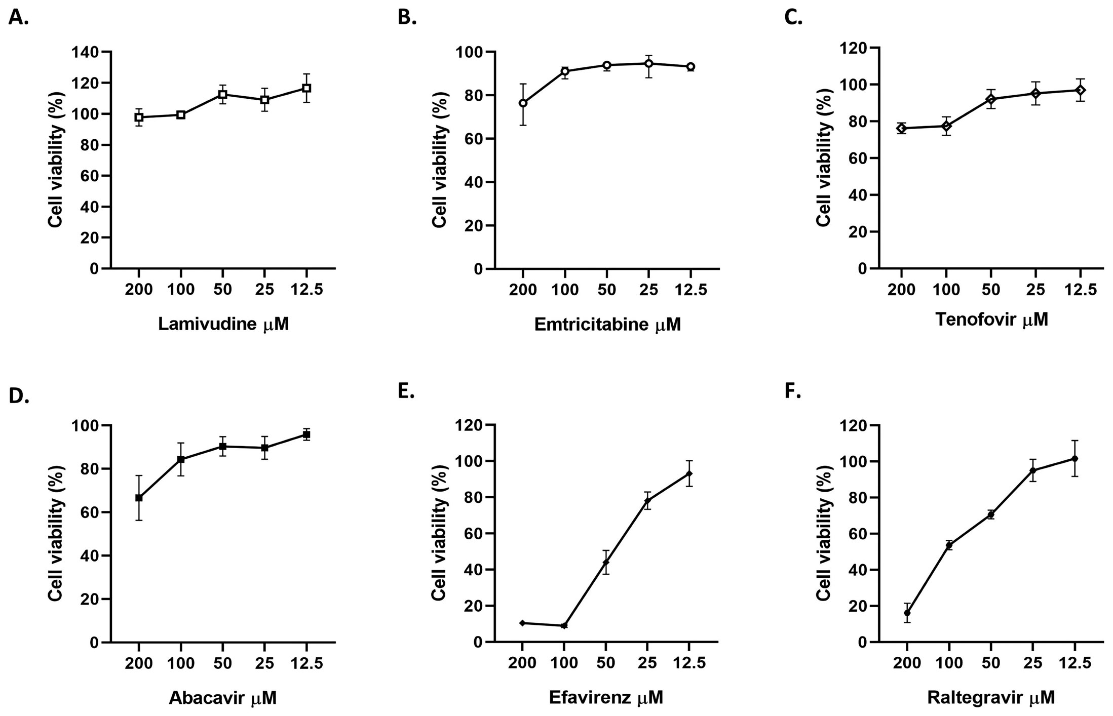
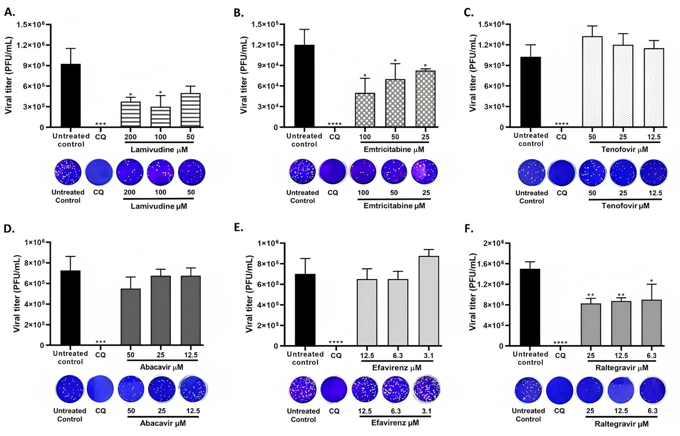
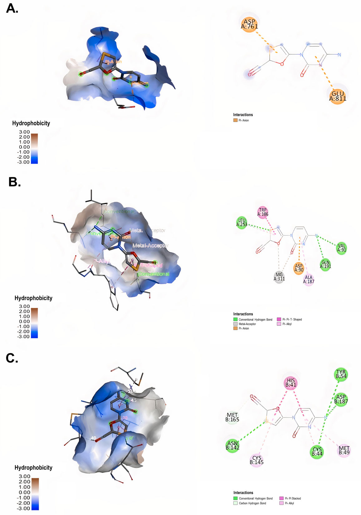
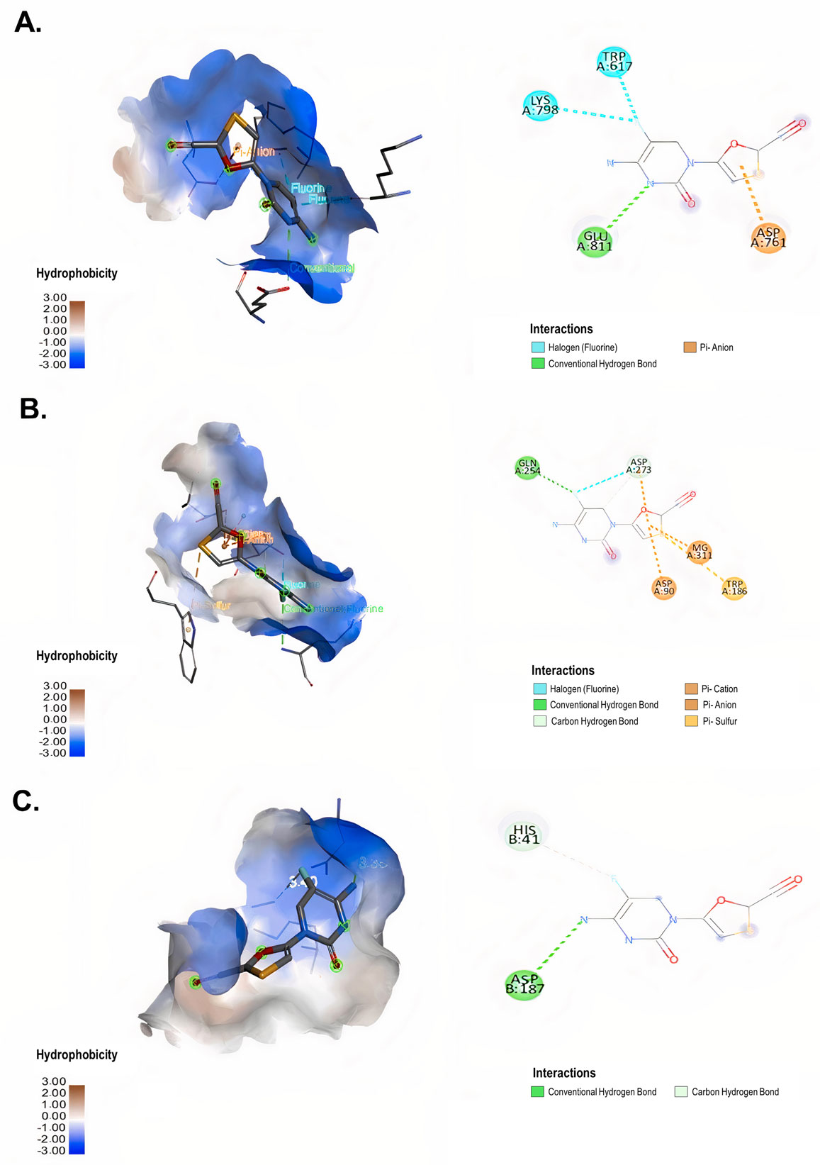
The cytotoxicity of lamivudine, emtricitabine, tenofovir, abacavir, efavirenz and raltegravir on Vero E6 was evaluated by MTT assay. The antiviral activity of each of these compounds was evaluated via a pre-post treatment strategy. The reduction in the viral titer was assessed by plaque assay. In addition, the affinities of the antiretroviral interaction with viral targets RdRp (RNA-dependent RNA polymerase), ExoN-NSP10 (exoribonuclease and its cofactor, the non-structural protein 10) complex and 3CLpro (3-chymotrypsin-like cysteine protease) were evaluated by molecular docking.
Results
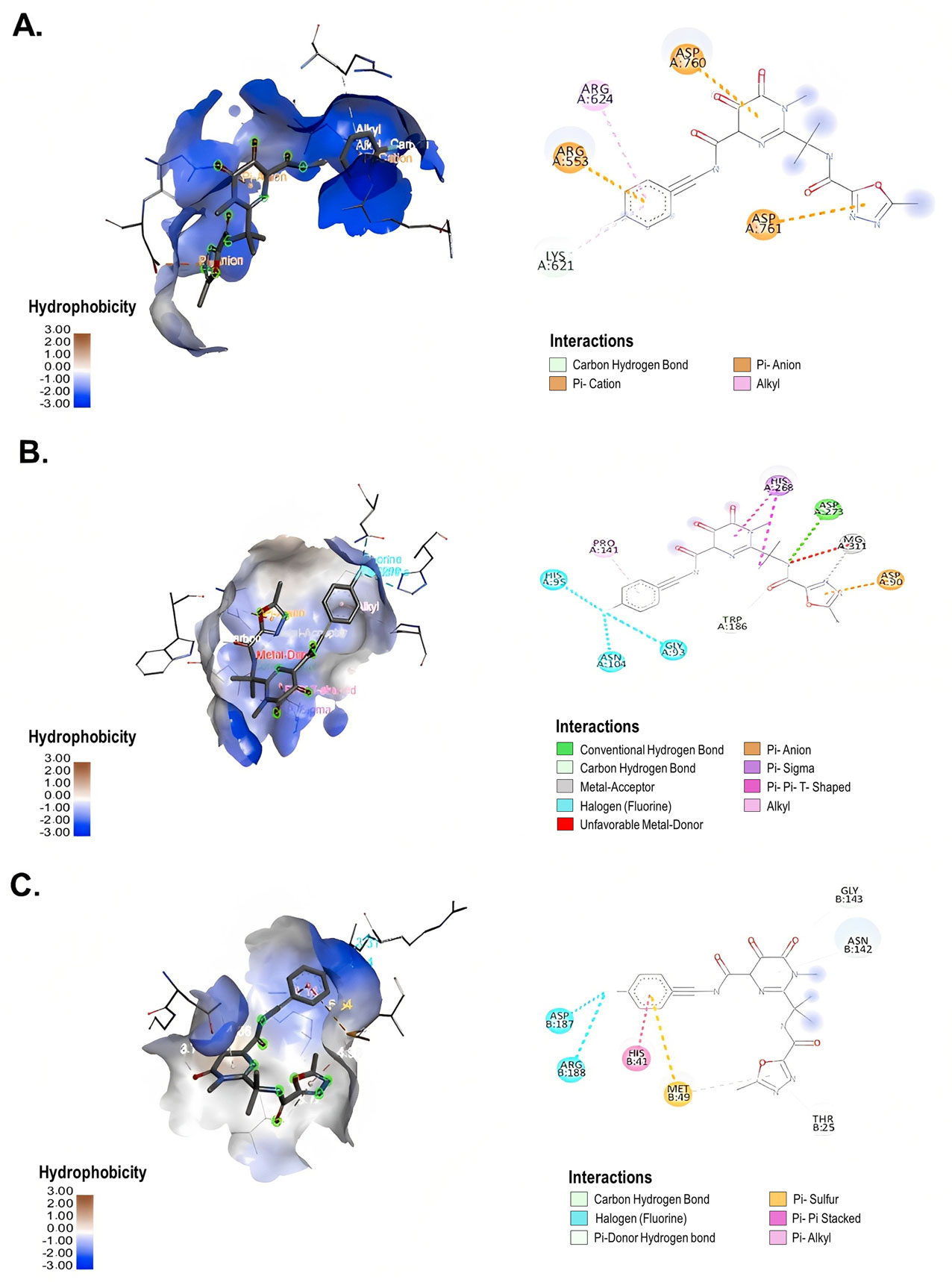
Lamivudine exhibited antiviral activity against SARS-CoV-2 at 200 µM (58.3%) and 100 µM (66.7%), while emtricitabine showed anti-SARS-CoV-2 activity at 100 µM (59.6%), 50 µM (43.4%) and 25 µM (33.3%). Raltegravir inhibited SARS-CoV-2 at 25, 12.5 and 6.3 µM (43.3%, 39.9% and 38.2%, respectively). The interaction between the antiretrovirals and SARS-CoV-2 RdRp, ExoN-NSP10 and 3CLpro yielded favorable binding energies (from −4.9 kcal/mol to −7.7 kcal/mol) using bioinformatics methods.
Conclusion
Lamivudine, emtricitabine and raltegravir showed in vitro antiviral effects against the D614G strain of SARS-CoV-2. Raltegravir was the compound with the greatest in vitro antiviral potential at low concentrations, and it showed the highest binding affinities with crucial SARS-CoV-2 proteins during the viral replication cycle. However, further studies on the therapeutic utility of raltegravir in patients with COVID-19 are required.
- antiretrovirals,
- SARS-CoV-2,
- COVID-19,
- molecular docking,
- drug repurposing
Citation: Maria I. Zapata-Cardona, Lizdany Florez-Alvarez, Ariadna L. Guerra-Sandoval, Mateo Chvatal-Medina, Carlos M. Guerra-Almonacid, Jaime Hincapie-Garcia, Juan C. Hernandez, Maria T. Rugeles, Wildeman Zapata-Builes. In vitro and in silico evaluation of antiretrovirals against SARS-CoV-2: A drug repurposing approach[J]. AIMS Microbiology, 2023, 9(1): 20-40. doi: 10.3934/microbiol.2023002

Related Papers:

Abstract

Background

Drug repurposing is a valuable strategy for rapidly developing drugs for treating COVID-19. This study aimed to evaluate the antiviral effect of six antiretrovirals against SARS-CoV-2 in vitro and in silico.

Methods

The cytotoxicity of lamivudine, emtricitabine, tenofovir, abacavir, efavirenz and raltegravir on Vero E6 was evaluated by MTT assay. The antiviral activity of each of these compounds was evaluated via a pre-post treatment strategy. The reduction in the viral titer was assessed by plaque assay. In addition, the affinities of the antiretroviral interaction with viral targets RdRp (RNA-dependent RNA polymerase), ExoN-NSP10 (exoribonuclease and its cofactor, the non-structural protein 10) complex and 3CLpro (3-chymotrypsin-like cysteine protease) were evaluated by molecular docking.

Results

Lamivudine exhibited antiviral activity against SARS-CoV-2 at 200 µM (58.3%) and 100 µM (66.7%), while emtricitabine showed anti-SARS-CoV-2 activity at 100 µM (59.6%), 50 µM (43.4%) and 25 µM (33.3%). Raltegravir inhibited SARS-CoV-2 at 25, 12.5 and 6.3 µM (43.3%, 39.9% and 38.2%, respectively). The interaction between the antiretrovirals and SARS-CoV-2 RdRp, ExoN-NSP10 and 3CLpro yielded favorable binding energies (from −4.9 kcal/mol to −7.7 kcal/mol) using bioinformatics methods.

Conclusion

Lamivudine, emtricitabine and raltegravir showed in vitro antiviral effects against the D614G strain of SARS-CoV-2. Raltegravir was the compound with the greatest in vitro antiviral potential at low concentrations, and it showed the highest binding affinities with crucial SARS-CoV-2 proteins during the viral replication cycle. However, further studies on the therapeutic utility of raltegravir in patients with COVID-19 are required.

Abbreviations

PDB ID

Protein Data Bank identification code

RdRp

RNA-dependent RNA polymerase

ExoN-NSP10

Exoribonuclease and its cofactor, the non-structural protein 10 complex

3CLpro

3-chymotrypsin-like cysteine protease

Acknowledgments

We want to thank to Instituto Nacional de Salud, Bogota-Colombia, for donating the Vero E6 cell line.

Conflicts of interest

The authors declare that the research was conducted in the absence of any commercial or financial relationships that could be construed as a potential conflict of interest. This study was supported by Universidad de Antioquia (strategy # UdeA responde al COVID-19), CODI (Act 2020–36850) and Universidad Cooperativa de Colombia. BPIN 2020000100131-SGR.

Author contributions

Study conception and design: MTR, WZB, CGA, AGS, JHG and JCH. Data collection, analysis and interpretation of results: MZC, LFA and AGS Draft manuscript preparation: MZC, LFA, AGS and MMC. Assistance with interpretation of the results and manuscript writing: MTR, WZB, CGA, JHG and JCH. Guide and review research: MTR and WZB. All authors have contributed to editing this paper; they have approved this final submission.

References

[1]	W.H.O.WHO Director-General' opening remarks at the media briefing on COVID-19-11 March 2020, 2020. Available from: https://www.who.int/director-general/speeches/detail/who-director-general-s-opening-remarks-at-the-media-briefing-on-covid-19---11-march-2020.
[2]	Lopera TJ, Chvatal-Medina M, Florez-Alvarez L, et al. (2022) Humoral response to BNT162b2 vaccine against SARS-CoV-2 variants decays after six months. Front Immunol 13: 879036. https://doi.org/10.3389/fimmu.2022.879036
[3]	Tada T, Zhou H, Dcosta BM, et al. (2021) Partial resistance of SARS-CoV-2 Delta variants to vaccine-elicited antibodies and convalescent sera. iScience 24: 103341. https://doi.org/10.1016/j.isci.2021.103341
[4]	Hoffmann M, Kruger N, Schulz S, et al. (2022) The Omicron variant is highly resistant against antibody-mediated neutralization: Implications for control of the COVID-19 pandemic. Cell 185: 447-456. https://doi.org/10.1016/j.cell.2021.12.032
[5]	Wang MY, Zhao R, Gao LJ, et al. (2020) SARS-CoV-2: structure, biology, and structure-based therapeutics development. Front Cell Infect Microbiol 10: 587269. https://doi.org/10.3389/fcimb.2020.587269
[6]	Yadav R, Chaudhary JK, Jain N, et al. (2021) Role of structural and non-structural proteins and therapeutic targets of SARS-CoV-2 for COVID-19. Cells 10: 821. https://doi.org/10.3390/cells10040821
[7]	Yang H, Rao Z (2021) Structural biology of SARS-CoV-2 and implications for therapeutic development. Nat Rev Microbiol 19: 685-700. https://doi.org/10.1038/s41579-021-00630-8
[8]	Gao Y, Yan L, Huang Y, et al. (2020) Structure of the RNA-dependent RNA polymerase from COVID-19 virus. Science 368: 779-782. https://doi.org/10.1126/science.abb7498
[9]	Lin S, Chen H, Chen Z, et al. (2021) Crystal structure of SARS-CoV-2 nsp10 bound to nsp14-ExoN domain reveals an exoribonuclease with both structural and functional integrity. Nucleic Acids Res 49: 5382-5392. https://doi.org/10.1093/nar/gkab320
[10]	Baddock H, Brolih S, Yosaatmadja Y, et al. (2022) Characterization of the SARS-CoV-2 ExoN (nsp14ExoN-nsp10) complex: implications for its role in viral genome stability and inhibitor identification. Nucleic Acids Res 50: 1484-1500. https://doi.org/10.1093/nar/gkab1303
[11]	V'kovski P, Kratzel A, Steiner S, et al. (2021) Coronavirus biology and replication: implications for SARS-CoV-2. Nat Rev Microbiol 19: 155-170. https://doi.org/10.1038/s41579-020-00468-6
[12]	Mosquera-Yuqui F, Lopez-Guerra N, Moncayo-Palacio EA (2020) Targeting the 3CLpro and RdRp of SARS-CoV-2 with phytochemicals from medicinal plants of the Andean Region: molecular docking and molecular dynamics simulations. J Biomol Struct Dyn 40: 2010-2023. https://doi.org/10.1080/07391102.2020.1835716
[13]	Peele KA, Potla Durthi C, Srihansa T, et al. (2020) Molecular docking and dynamic simulations for antiviral compounds against SARS-CoV-2: A computational study. Inform Med Unlocked 19: 100345. https://doi.org/10.1016/j.imu.2020.100345
[14]	Cao B, Wang Y, Wen D, et al. (2020) A trial of lopinavir–ritonavir in adults hospitalized with severe Covid-19. N Engl J Med 382: 1787-1799. https://doi.org/10.1056/NEJMoa2001282
[15]	Arabi YM, Gordon AC, Derde LPG, et al. (2021) Lopinavir-ritonavir and hydroxychloroquine for critically ill patients with COVID-19: REMAP-CAP randomized controlled trial. Intensive Care Med 47: 867-886. https://doi.org/10.1007/s00134-021-06448-5
[16]	Beck BR, Shin B, Choi Y, et al. (2020) Predicting commercially available antiviral drugs that may act on the novel coronavirus (SARS-CoV-2) through a drug-target interaction deep learning model. Comput Struct Biotechnol J 18: 784-790. https://doi.org/10.1016/j.csbj.2020.03.025
[17]	Jordaan MA, Ebenezer O, Damoyi N, et al. (2020) Virtual screening, molecular docking studies and DFT calculations of FDA approved compounds similar to the non-nucleoside reverse transcriptase inhibitor (NNRTI) efavirenz. Heliyon 6: e04642. https://doi.org/10.1016/j.heliyon.2020.e04642
[18]	Indu P, Rameshkumar MR, Arunagirinathan N, et al. (2020) Raltegravir, Indinavir, Tipranavir, Dolutegravir, and Etravirine against main protease and RNA-dependent RNA polymerase of SARS-CoV-2: A molecular docking and drug repurposing approach. J Infect Public Health 13: 1856-1861. https://doi.org/10.1016/j.jiph.2020.10.015
[19]	Jockusch S, Tao C, Li X, et al. (2020) Triphosphates of the Two Components in DESCOVY and TRUVADA are Inhibitors of the SARS-CoV-2 Polymerase. bioRxiv : 2020. https://doi.org/10.1101/2020.04.03.022939
[20]	Alavian G, Kolahdouzan K, Mortezazadeh M, et al. (2021) Antiretrovirals for Prophylaxis Against COVID-19: A Comprehensive Literature Review. J Clin Pharmacol 61: 581-590. https://doi.org/10.1002/jcph.1788
[21]	Arts EJ, Hazuda DJ (2012) HIV-1 antiretroviral drug therapy. Cold Spring Harb Perspect Med 2: a007161. https://doi.org/10.1101/cshperspect.a007161
[22]	Kumar Y, Singh H, Patel CN (2020) In silico prediction of potential inhibitors for the main protease of SARS-CoV-2 using molecular docking and dynamics simulation based drug-repurposing. J Infect Public Health 13: 1210-1223. https://doi.org/10.1016/j.jiph.2020.06.016
[23]	Jo S, Kim S, Yoo J, et al. (2021) A study of 3CLpros as promising targets against SARS-CoV and SARS-CoV-2. Microorganisms 9: 756. https://doi.org/10.3390/microorganisms9040756
[24]	Garcia-Trejo JJ, Ortega R, Zarco-Zavala M (2021) Putative repurposing of lamivudine, a nucleoside/nucleotide analogue and antiretroviral to improve the outcome of cancer and COVID-19 patients. Front Oncol 11: 664794. https://doi.org/10.3389/fonc.2021.664794
[25]	Clososki CG, Soldi RA, Moreira Silva R, et al. (2020) Tenofovir disoproxil fumarate: new chemical developments and encouraging in vitro biological results for SARS-CoV-2. J Braz Chem Soc 31: 1552-1556. https://doi.org/10.21577/0103-5053.20200106
[26]	Copertino D, Lima B, Duarte R, et al. (2020) Antiretroviral drug activity and potential for pre-exposure prophylaxis against COVID-19 and HIV infection. J Biomol Struct Dyn 40: 7367-7380. https://doi.org/10.26434/chemrxiv.12250199
[27]	Chien M, Anderson TK, Jockusch S, et al. (2020) Nucleotide analogues as inhibitors of SARS-CoV-2 polymerase, a key drug target for COVID-19. J Proteome Res 19: 4690-4697. https://doi.org/10.1021/acs.jproteome.0c00392
[28]	Xie X, Muruato AE, Zhang X, et al. (2020) A nanoluciferase SARS-CoV-2 for rapid neutralization testing and screening of anti-infective drugs for COVID-19. Nat Commun 11: 5214. https://doi.org/10.1038/s41467-020-19055-7
[29]	Martinec O, Huliciak M, Staud F, et al. (2019) Anti-HIV and anti-Hepatitis C virus drugs inhibit P-Glycoprotein efflux activity in Caco-2 Cells and precision-cut rat and human intestinal slices. Antimicrob Agents Chemother 63: e00910-00919. https://doi.org/10.1128/aac.00910-19
[30]	Cong Y, Dyall J, Hart BJ, et al. (2016) Evaluation of the activity of lamivudine and zidovudine against Ebola virus. PLoS One 11: e0166318. https://doi.org/10.1371/journal.pone.0166318
[31]	Zang R, Case JB, Yutuc E, et al. (2020) Cholesterol 25-hydroxylase suppresses SARS-CoV-2 replication by blocking membrane fusion. Proc Natl Acad Sci U S A 117: 32105-32113. https://doi.org/10.1073/pnas.2012197117
[32]	Diaz FJ, Aguilar-Jimenez W, Florez-Alvarez L, et al. (2020) Isolation and characterization of an early SARS-CoV-2 isolate from the 2020 epidemic in Medellin, Colombia. Biomedica 40: 148-158. https://doi.org/10.7705/biomedica.5834
[33]	Chosewood L, Wilson D (2009) Biosafety in Microbiological and Biomedical Laboratories.US Department of Health and Human Services: 415.
[34]	Zapata-Cardona MI, Florez-Alvarez L, Zapata-Builes W, et al. (2022) Atorvastatin effectively inhibits ancestral and two emerging variants of SARS-CoV-2 in vitro. Front Microbiol 13: 721103. https://doi.org/10.3389/fmicb.2022.721103
[35]	Marin-Palma D, Tabares-Guevara JH, Zapata-Cardona MI, et al. (2021) Curcumin inhibits in vitro SARS-CoV-2 infection in vero E6 cells through multiple antiviral mechanisms. Molecules 26: 6900. https://doi.org/10.3390/molecules26226900
[36]	Zapata Cardona M, Florez-Alvarez L, Gomez-Gallego D, et al. (2022) Comparison among plaque assay, tissue culture infectious dose (TCID50) and real-time RT-PCR for SARS-CoV-2 variants quantification. Iran J Microbiol 14: 291-299. https://doi.org/10.18502/ijm.v14i3.9758
[37]	Moeller NH, Shi K, Demir O, et al. (2021) Structure and dynamics of SARS-CoV-2 proofreading exoribonuclease ExoN. bioRxiv . https://doi.org/10.1101/2021.04.02.438274
[38]	Su HX, Yao S, Zhao WF, et al. (2020) Anti-SARS-CoV-2 activities in vitro of Shuanghuanglian preparations and bioactive ingredients. Acta Pharmacol Sin 41: 1167-1177. https://doi.org/10.1038/s41401-020-0483-6
[39]	Berman HM, Westbrook J, Feng Z, et al. (2020) The protein data bank. Nucleic Acids Res 28: 235-242. https://doi.org/10.1093/nar/28.1.235
[40]	Curry S (2015) Structural biology: a century-long journey into an unseen world. Interdiscip Sci Rev 40: 308-328. https://doi.org/10.1179/0308018815Z.000000000120
[41]	BIOVIA DSDiscovery studio visualizer software, version 16.1 2017. Available from: https://discover.3ds.com/discovery-studio-visualizer-download.
[42]	Chu CK, Gadthula S, Chen X, et al. (2006) Antiviral activity of nucleoside analogues against SARS-coronavirus (SARS-CoV). Antivir Chem Chemother 17: 285-289. https://doi.org/10.1177/095632020601700506
[43]	Hanwell MD, Curtis DE, Lonie DC, et al. (2012) Avogadro: an advanced semantic chemical editor, visualization, and analysis platform. J Cheminformatics 4: 17. https://doi.org/10.1186/1758-2946-4-17
[44]	Kokic G, Hillen HS, Tegunov D, et al. (2021) Mechanism of SARS-CoV-2 polymerase stalling by remdesivir. Nat Commun 12: 279. https://doi.org/10.1038/s41467-020-20542-0
[45]	Koulgi S, Jani V, Uppuladinne M, et al. (2020) Remdesivir-bound and ligand-free simulations reveal the probable mechanism of inhibiting the RNA dependent RNA polymerase of severe acute respiratory syndrome coronavirus 2. RSC Advances 10: 26792-26803. https://doi.org/10.1039/D0RA04743K
[46]	Wang X, Sacramento CQ, Jockusch S, et al. (2022) Combination of antiviral drugs inhibits SARS-CoV-2 polymerase and exonuclease and demonstrates COVID-19 therapeutic potential in viral cell culture. Commun Biol 5: 154. https://doi.org/10.1038/s42003-022-03101-9
[47]	Nimgampalle M, Devanathan V, Saxena A (2020) Screening of Chloroquine, Hydroxychloroquine and its derivatives for their binding affinity to multiple SARS-CoV-2 protein drug targets. J Biomol Struct Dyn : 1-13. https://doi.org/10.1080/07391102.2020.1782265
[48]	Li Z, Li X, Huang YY, et al. (2020) Identify potent SARS-CoV-2 main protease inhibitors via accelerated free energy perturbation-based virtual screening of existing drugs. Proc Natl Acad Sci USA 117: 27381. https://doi.org/10.1073/pnas.2010470117
[49]	Jendele L, Krivak R, Skoda P, et al. (2019) PrankWeb: a web server for ligand binding site prediction and visualization. Nucleic Acids Res 47: W345-W349. https://doi.org/10.1093/nar/gkz424
[50]	Schoning-Stierand K, Diedrich K, Fahrrolfes R, et al. (2020) ProteinsPlus: interactive analysis of protein–ligand binding interfaces. Nucleic Acids Res 48: W48-W53. https://doi.org/10.1093/nar/gkaa235
[51]	Elfiky AA (2020) Ribavirin, Remdesivir, Sofosbuvir, Galidesivir, and Tenofovir against SARS-CoV-2 RNA dependent RNA polymerase (RdRp): A molecular docking study. Life Sci 253: 117592. https://doi.org/10.1016/j.lfs.2020.117592
[52]	Narayanan N, Nair DT (2021) Ritonavir may inhibit exoribonuclease activity of nsp14 from the SARS-CoV-2 virus and potentiate the activity of chain terminating drugs. Int J Biol Macromol 168: 272-278. https://doi.org/10.1016/j.ijbiomac.2020.12.038
[53]	Trott O, Olson AJ (2010) AutoDock Vina: improving the speed and accuracy of docking with a new scoring function, efficient optimization, and multithreading. J Comput Chem 31: 455-461. https://doi.org/10.1002/jcc.21334
[54]	Ma Y, Wu L, Shaw N, et al. (2015) Structural basis and functional analysis of the SARS coronavirus nsp14-nsp10 complex. Proc Natl Acad Sci USA 112: 9436-9441. https://doi.org/10.1073/pnas.1508686112
[55]	Frediansyah A, Tiwari R, Sharun K, et al. (2021) Antivirals for COVID-19: a critical review. Clin Epidemiol Glob Health 9: 90-98. https://doi.org/10.1016/j.cegh.2020.07.006
[56]	Iacob S, Iacob DG (2020) SARS-CoV-2 Treatment approaches: numerous ptions, no certainty for a versatile virus. Front Pharmacol 11. https://doi.org/10.3389/fphar.2020.01224
[57]	Papatheodoridis GV, Dimou E, Papadimitropoulos V (2002) Nucleoside analogues for chronic hepatitis B: antiviral efficacy and viral resistance. Am J Gastroenterol 97: 1618-1628. https://doi.org/10.1111/j.1572-0241.2002.05819.x
[58]	Joly V, Yeni P (1995) Treatment of HIV infection with nucleoside analogs: present status. Presse Med 24: 103-110.
[59]	Furman PA, Lam AM, Murakami E (2009) Nucleoside analog inhibitors of hepatitis C viral replication: recent advances, challenges and trends. Future Med Chem 1: 1429-1452. https://doi.org/10.4155/fmc.09.88
[60]	Fiala M, Chow AW, Miyasaki K, et al. (1974) Susceptibility of herpesviruses to three nucleoside analogues and their combinations and enhancement of the antiviral effect at acid pH. J Infect Dis 129: 82-85. https://doi.org/10.1093/infdis/129.1.82
[61]	Lisi L, Lacal PM, Barbaccia ML, et al. (2020) Approaching coronavirus disease 2019: mechanisms of action of repurposed drugs with potential activity against SARS-CoV-2. Biochem Pharmacol 180: 11416. https://doi.org/10.1016/j.bcp.2020.114169
[62]	Smith EC, Blanc H, Surdel MC, et al. (2013) Coronaviruses lacking exoribonuclease activity are susceptible to lethal mutagenesis: evidence for proofreading and potential therapeutics. PLoS pathogens 9: e100356. https://doi.org/10.1371/journal.ppat.1003565
[63]	Agostini ML, Andres EL, Sims AC, et al. (2018) Coronavirus susceptibility to the antiviral remdesivir (GS-5734) is mediated by the viral polymerase and the proofreading exoribonuclease. mBio 9: e00221-00218. https://doi.org/10.1128/mBio.00221-18
[64]	Tran L, Tam DNH, Elhadad H, et al. (2022) Evaluation of COVID-19 protease and HIV inhibitors interactions. Acta Pharm 72: 1-8. https://doi.org/10.2478/acph-2022-0010
[65]	Ullrich S, Nitsche C (2020) The SARS-CoV-2 main protease as drug target. Bioorganic Med Chem Lett 30: 127377. https://doi.org/10.1016/j.bmcl.2020.127377
[66]	Pinzi L, Rastelli G (2019) Molecular docking: shifting paradigms in drug discovery. Int J Mol Sci 20: 4331. https://doi.org/10.3390/ijms20184331
[67]	Coupez B, Lewis RA (2006) Docking and scoring--theoretically easy, practically impossible?. Curr Med Chem 13: 2995-3003. https://doi.org/10.2174/092986706778521797
[68]	Guedes IA, Pereira FSS, Dardenne LE (2018) Empirical scoring functions for structure-based virtual screening: applications, critical aspects, and challenges. Front Pharmacol 9: 1089. https://doi.org/10.3389/fphar.2018.01089
[69]	Pruijssers AJ, George AS, Schafer A, et al. (2020) Remdesivir inhibits SARS-CoV-2 in human lung cells and chimeric SARS-CoV expressing the SARS-CoV-2 RNA polymerase in mice. Cell Rep 32: 107940. https://doi.org/10.1016/j.celrep.2020.107940
[70]	Pruijssers AJ, Denison MR (2019) Nucleoside analogues for the treatment of coronavirus infections. Curr Opin Virol 35: 57-62. https://doi.org/10.1016/j.coviro.2019.04.002
[71]	Koczor CA, Torres RA, Lewis W (2012) The role of transporters in the toxicity of nucleoside and nucleotide analogs. Expert Opin Drug Metab Toxicol 8: 665-676. https://doi.org/10.1517/17425255.2012.680885
[72]	Eyer L, Nencka R, de Clercq E, et al. (2018) Nucleoside analogs as a rich source of antiviral agents active against arthropod-borne flaviviruses. Antivir Chem Chemother 26: 2040206618761299. https://doi.org/10.1177/2040206618761299
[73]	He X, Quan S, Xu M, et al. (2021) Generation of SARS-CoV-2 reporter replicon for high-throughput antiviral screening and testing. Proc Natl Acad Sci USA 118: e2025866118. https://doi.org/10.1073/pnas.2025866118
[74]	Sankatsing SU, Beijnen JH, Schinkel AH, et al. (2004) P glycoprotein in human immunodeficiency virus type 1 infection and therapy. Antimicrob Agents Chemother 48: 1073-1081. https://doi.org/10.1128/aac.48.4.1073-1081.2004
[75]	ClinicalTrials.govClinical Experimentation With Tenofovir Disoproxyl Fumarate and Emtricitabine for COVID-19 (ARTAN-C19) (2021). Available from: https://clinicaltrials.gov/ct2/show/NCT04712357?term=emtricitabine&cond=covid 19&draw=2&rank=1.
[76]	ClinicalTrials.govClinical trial to evaluate the efficacy of different treatments in patients with COVID-19 (2021). Available from: https://clinicaltrials.gov/ct2/show/NCT04890626?term=emtricitabine&cond=covid-19&draw=2.
[77]	ClinicalTrials.govDaily regimen of tenofovir/emtricitabine as prevention for COVID-19 in health care personnel in Colombia (2020). Available from: https://clinicaltrials.gov/ct2/show/NCT04519125?term=emtricitabine&cond=covid-19&draw=2&rank=3.
[78]	Parienti JJ, Prazuck T, Peyro-Saint-Paul L, et al. (2021) Effect of tenofovir disoproxil fumarate and emtricitabine on nasopharyngeal SARS-CoV-2 viral load burden amongst outpatients with COVID-19: A pilot, randomized, open-label phase 2 trial. EClinicalMedicine 38: 100993. https://doi.org/10.1016/j.eclinm.2021.100993
[79]	Gaitan-Duarte HG, Alvarez-Moreno C, Rincon-Rodriguez CJ, et al. (2022) Effectiveness of rosuvastatin plus colchicine, emtricitabine/tenofovir and combinations thereof in hospitalized patients with COVID-19: a pragmatic, open-label randomized trial. EClinicalMedicine 43: 101242. https://doi.org/10.1016/j.eclinm.2021.101242
[80]	Del Amo J, Polo R, Moreno S, et al. (2020) Incidence and severity of COVID-19 in HIV-positive persons receiving antiretroviral therapy: a cohort study. Ann Intern Med 173: 536-541. https://doi.org/10.7326/M20-3689
[81]	Moss DM, Kwan WS, Liptrott NJ, et al. (2011) Raltegravir is a substrate for SLC22A6: a putative mechanism for the interaction between raltegravir and tenofovir. Antimicrob Agents Chemother 55: 879-887. https://doi.org/10.1128/AAC.00623-10
[82]	Khan RJ, Jha RK, Amera GM, et al. (2021) Targeting SARS-CoV-2: a systematic drug repurposing approach to identify promising inhibitors against 3C-like proteinase and 2′-O-ribose methyltransferase. J Biomol Struct Dyn 39: 2679-2692. https://doi.org/10.1080/07391102.2020.1753577
[83]	Molavi Z, Razi S, Mirmotalebisohi SA, et al. (2021) Identification of FDA approved drugs against SARS-CoV-2 RNA dependent RNA polymerase (RdRp) and 3-chymotrypsin-like protease (3CLpro), drug repurposing approach. Biomed Pharmacother 138: 111544. https://doi.org/10.1016/j.biopha.2021.111544
[84]	Tazikeh-Lemeski E, Moradi S, Raoufi R, et al. (2021) Targeting SARS-COV-2 non-structural protein 16: a virtual drug repurposing study. J Biomol Struct Dyn 39: 4633-4646. https://doi.org/10.1080/07391102.2020.1779133

microbiol-09-01-002-s001.pdf

Reader Comments

Your name:*

Email:*
© 2023 the Author(s), licensee AIMS Press. This is an open access article distributed under the terms of the Creative Commons Attribution License (http://creativecommons.org/licenses/by/4.0)