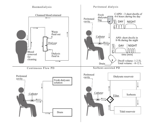
Peritoneal dialysis (PD) is a kidney replacement therapy for patients with end-stage renal disease. It is becoming more popular as a result of a rising interest in home dialysis. Its effectiveness depends on several physiological and technical factors, which have led to the development of various computational models to better understand and predict PD outcomes. In this review, we traced the evolution of computational PD models, discussed the principles underlying these models, including the transport kinetics of solutes, the fluid dynamics within the peritoneal cavity, and the peritoneal membrane properties, and reviewed the various PD models that can be used to optimize and personalize PD treatment. By providing a comprehensive overview, we aim to guide both current clinical practice and future research into novel PD techniques such as the application of continuous flow and sorbent-based dialysate regeneration where mathematical modeling may offer an inexpensive and effective tool to optimize design of these novel techniques at a patient specific level.
Citation: Sangita Swapnasrita, Joost C de Vries, Carl M. Öberg, Aurélie MF Carlier, Karin GF Gerritsen. Computational modeling of peritoneal dialysis: An overview[J]. Mathematical Biosciences and Engineering, 2025, 22(2): 431-476. doi: 10.3934/mbe.2025017
Peritoneal dialysis (PD) is a kidney replacement therapy for patients with end-stage renal disease. It is becoming more popular as a result of a rising interest in home dialysis. Its effectiveness depends on several physiological and technical factors, which have led to the development of various computational models to better understand and predict PD outcomes. In this review, we traced the evolution of computational PD models, discussed the principles underlying these models, including the transport kinetics of solutes, the fluid dynamics within the peritoneal cavity, and the peritoneal membrane properties, and reviewed the various PD models that can be used to optimize and personalize PD treatment. By providing a comprehensive overview, we aim to guide both current clinical practice and future research into novel PD techniques such as the application of continuous flow and sorbent-based dialysate regeneration where mathematical modeling may offer an inexpensive and effective tool to optimize design of these novel techniques at a patient specific level.

| [1] |
K. J. Jager, C. Kovesdy, R. Langham, M. Rosenberg, V. Jha, C. Zoccali, A single number for advocacy and communication—worldwide more than 850 million individuals have kidney diseases, Nephrol. Dial. Transplant., 34 (2019), 1803–1805. https://doi.org/10.1093/ndt/gfz174 doi: 10.1093/ndt/gfz174

|
| [2] | Fresenius Medical Care Annual Report, (2021), 39–40. |
| [3] |
M. Bonomini, V. Zammit, J. C. Divino-Filho, S. J. Davies, L. Di Liberato, A. Arduini, et al., The osmo-metabolic approach: a novel and tantalizing glucose-sparing strategy in peritoneal dialysis, J. Nephrol., 34 (2021), 503–519. https://doi.org/10.1007/s40620-020-00804-2 doi: 10.1007/s40620-020-00804-2
|
| [4] |
P. Freida, M. Galach, J. C. D. Filho, A. Werynski, B. Lindholm, Combination of crystalloid (glucose) and colloid (icodextrin) osmotic agents markedly enhances peritoneal fluid and solute transport during the long PD dwell, Perit. Dial. Int., 27 (2007), 267–276. https://doi.org/10.1177/089686080702700311 doi: 10.1177/089686080702700311
|
| [5] |
K. Nishimura, Y. Kamiya, K. Miyamoto, S. Nomura, T. Horiuchi, Molecular weight of polydisperse icodextrin effects its oncotic contribution to water transport, J. Artif. Organs, 11 (2008), 165–169. https://doi.org/10.1007/s10047-008-0423-6 doi: 10.1007/s10047-008-0423-6
|
| [6] |
J. Stachowska-Pietka, J. Waniewski, A. Olszowska, E. Garcia-Lopez, J. Yan, Q. Yao, et al., Can one long peritoneal dwell with icodextrin replace two short dwells with glucose?, Front. Physiol., 15 (2024). https://doi.org/10.3389/fphys.2024.1339762 doi: 10.3389/fphys.2024.1339762
|
| [7] |
B. Rippe, G. Stelin, B. Haraldsson, Computer simulations of peritoneal fluid transport in CAPD, Kidney Int., 40 (1991), 315–325. https://doi.org/10.1038/ki.1991.216 doi: 10.1038/ki.1991.216
|
| [8] |
R. P. Popovich, J. W. Moncrief, K. D. Nolph, A. J. Ghods, Z. J. Twardowski, W. K. Pyle, Continuous ambulatory peritoneal dialysis, Ann. Intern. Med., 88 (1978), 449–456. https://doi.org/10.7326/0003-4819-88-4-449 doi: 10.7326/0003-4819-88-4-449
|
| [9] |
T. A. Golper, R. Chaudhry, Automated cyclers used in peritoneal dialysis: technical aspects for the clinician, Med. Devices: Evidence Res., (2015), 95. https://doi.org/10.2147/mder.s51189 doi: 10.2147/mder.s51189
|
| [10] |
B. Marrón, C. Remón, M. Pérez-Fontán, P. Quirós, A. Ortíz, Benefits of preserving residual renal function in peritoneal dialysis, Kidney Int., 73 (2008), S42–S51. https://doi.org/10.1038/sj.ki.5002600 doi: 10.1038/sj.ki.5002600
|
| [11] |
B. G. Jaar, L. C. Plantinga, D. C. Crews, N. E. Fink, N. Hebah, J. Coresh, et al., Timing, causes, predictors and prognosis of switching from peritoneal dialysis to hemodialysis: A prospective study, BMC Nephrol., 10 (2009), 3. https://doi.org/10.1186/1471-2369-10-3 doi: 10.1186/1471-2369-10-3
|
| [12] |
A. A. Bonenkamp, A. V. E. V. Der Sluijs, F. W. Dekker, D. G. Struijk, C. W. H. De Fijter, Y. M. Vermeeren, et al., Technique failure in peritoneal dialysis: Modifiable causes and patient-specific risk factors, Perit. Dial. Int., (2022), 08968608221077461. https://doi.org/10.1177/08968608221077461 doi: 10.1177/08968608221077461
|
| [13] |
A. Van Eck Van Der Sluijs, A. A. Bonenkamp, F. W. Dekker, A. C. Abrahams, B. C. Van Jaarsveld, A. C. Abrahams, et al., Dutch nOcturnal and hoME dialysis Study To Improve Clinical Outcomes (DOMESTICO): rationale and design, BMC Nephrol., 20 (2019), 361. https://doi.org/10.1186/s12882-019-1526-4 doi: 10.1186/s12882-019-1526-4
|
| [14] | Nefrovisie, www.nefrovisie.nl |
| [15] |
T. T. Jansz, M. Noordzij, A. Kramer, E. Laruelle, C. Couchoud, F. Collart, et al., Survival of patients treated with extended-hours haemodialysis in Europe: an analysis of the ERA-EDTA Registry, Nephrol. Dial. Transplant., 35 (2020), 488–495. https://doi.org/10.1093/ndt/gfz208 doi: 10.1093/ndt/gfz208
|
| [16] |
A. W. Y. Yu, K. F. Chau, Y. W. Ho, P. K. T. Li, Development of the "peritoneal dialysis first" model in Hong Kong, Perit. Dial. Int., 27 (2007), 53–55. https://doi.org/10.1177/089686080702702s09 doi: 10.1177/089686080702702s09
|
| [17] |
C. Ronco, R. Amerling, Continuous flow peritoneal dialysis: current state-of-the-art and obstacles to further development, Contrib. Nephrol., 150 (2006), 310–320. https://doi.org/10.1159/000093625 doi: 10.1159/000093625
|
| [18] |
R. Amerling, J. F. Winchester, C. Ronco, Continuous flow peritoneal dialysis: update 2012, Contrib. Nephrol., 178 (2012), 205–215. https://doi.org/10.1159/000337854 doi: 10.1159/000337854
|
| [19] |
M. K. Van Gelder, J. C. De Vries, F. Simonis, A. S. Monninkhof, D. H. M. Hazenbrink, G. Ligabue, et al., Evaluation of a system for sorbent‐assisted peritoneal dialysis in a uremic pig model, Physiol. Rep., 8 (2020), e14593. https://doi.org/10.14814/phy2.14593 doi: 10.14814/phy2.14593
|
| [20] |
M. K. Van Gelder, G. Ligabue, S. Giovanella, E. Bianchini, F. Simonis, D. H. M. Hazenbrink, et al., In vitro efficacy and safety of a system for sorbent-assisted peritoneal dialysis, Am. J. Physiol. Renal. Physiol., 319 (2020), F162–F170. https://doi.org/10.1152/ajprenal.00079.2020 doi: 10.1152/ajprenal.00079.2020
|
| [21] |
K. Gerritsen, WEAKID - Clinical validation of miniature wearable dialysis machine - H2020, Impact, 2018 (2018), 55–57. https://doi.org/10.21820/23987073.2018.3.55 doi: 10.21820/23987073.2018.3.55
|
| [22] |
R. Herzog, M. Bartosova, S. Tarantino, A. Wagner, M. Unterwurzacher, J. M. Sacnun, et al., Peritoneal dialysis fluid supplementation with alanyl-glutamine attenuates conventional dialysis fluid-mediated endothelial cell injury by restoring perturbed cytoprotective responses, Biomolecules, 10 (2020). https://doi.org/10.3390/biom10121678 doi: 10.3390/biom10121678
|
| [23] |
P. Freida, M. Wilkie, S. Jenkins, F. Dallas, B. Issad, The contribution of combined crystalloid and colloid osmosis to fluid and sodium management in peritoneal dialysis, Kidney Int., 73 (2008), S102–S111. https://doi.org/10.1038/sj.ki.5002610 doi: 10.1038/sj.ki.5002610
|
| [24] |
S. Jenkins, M. Wilkie, Mixing osmotic agents–two different approaches, Perit. Dial. Int., 27 (2007), 245–250. https://doi.org/10.1177/089686080702700306 doi: 10.1177/089686080702700306
|
| [25] |
R. Amerling, C. Ronco, N. W. Levin, Continuous-flow peritoneal dialysis, Perit. Dial. Int., 20 (2000), 172–177. https://doi.org/10.1177/089686080002002S32 doi: 10.1177/089686080002002S32
|
| [26] |
J. A. Diaz-Buxo, Evolution of continuous flow peritoneal dialysis and the current state of the art, Semin. Dial., 14 (2001), 373–377. https://doi.org/10.1046/j.1525-139X.2001.00097.x doi: 10.1046/j.1525-139X.2001.00097.x
|
| [27] |
J. Winchester, R. Amerling, N. Harbord, V. Capponi, C. Ronco, The potential application of sorbents in peritoneal dialysis, Contrib. Nephrol., 150 (2006), 336–343. https://doi.org/10.1159/000093628 doi: 10.1159/000093628
|
| [28] |
M. Roberts, The regenerative dialysis (REDY) sorbent system, Nephrology, 4 (1998), 275–278. https://doi.org/https://doi.org/10.1111/j.1440-1797.1998.tb00359.x doi: 10.1111/j.1440-1797.1998.tb00359.x
|
| [29] |
E. A. M. Neugebauer, A. Rath, S. L. Antoine, M. Eikermann, D. Seidel, C. Koenen, et al., Specific barriers to the conduct of randomised clinical trials on medical devices, Trials, 18 (2017), 427. https://doi.org/10.1186/s13063-017-2168-0 doi: 10.1186/s13063-017-2168-0
|
| [30] |
C. A. Labarrere, A. E. Dabiri, G. S. Kassab, Thrombogenic and inflammatory reactions to biomaterials in medical devices, Front. Bioeng. Biotech., 8 (2020). https://doi.org/10.3389/fbioe.2020.00123 doi: 10.3389/fbioe.2020.00123
|
| [31] |
M. Zilberman, A. Malka, Drug controlled release from structured bioresorbable films used in medical devices—A mathematical model, J. Biomed. Mater. Res. B Appl. Biomater, 89B (2009), 155–164. https://doi.org/10.1002/jbm.b.31200 doi: 10.1002/jbm.b.31200
|
| [32] |
B. Ercan, D. Khang, J. Carpenter, T. J. Webster, Using mathematical models to understand the effect of nanoscale roughness on protein adsorption for improving medical devices, Int J Nanomedicine, 8 Suppl 1 (2013), 75–81. https://doi.org/10.2147/IJN.S47286 doi: 10.2147/IJN.S47286
|
| [33] |
Y. Wang, Y. Zou, X. Chen, J. Zhu, C. Xiang, H. Jia, et al., Identification of the appropriate fixation site to avoid peritoneal catheter migration based on a mechanical analysis, Ren. Fail., 39 (2017), 400–405. https://doi.org/10.1080/0886022X.2017.1291433 doi: 10.1080/0886022X.2017.1291433
|
| [34] | E. G. Galli, C. Taietti, M. Borghi, Personalization of automated peritoneal dialysis treatment using a computer modeling system, Adv. Perit. Dial., 27 (2011), 90–96. |
| [35] |
J. W. Yates, R. O. Jones, M. Walker, S. A. Cheung, Structural identifiability and indistinguishability of compartmental models, Expert Opin. Drug Metab. Toxicol., 5 (2009), 295–302. https://doi.org/10.1517/17425250902773426 doi: 10.1517/17425250902773426
|
| [36] |
J. King, K. S. Eroumé, R. Truckenmüller, S. Giselbrecht, A. E. Cowan, L. Loew, et al., Ten steps to investigate a cellular system with mathematical modeling, PLoS Comput. Biol., 17 (2021), e1008921. https://doi.org/10.1371/journal.pcbi.1008921 doi: 10.1371/journal.pcbi.1008921
|
| [37] |
R. F. Brown, Compartmental system analysis: State of the art, IEEE Trans. Biomed. Eng., BME-27 (1980), 1–11. https://doi.org/10.1109/TBME.1980.326685 doi: 10.1109/TBME.1980.326685
|
| [38] |
C. M. Öberg, G. Martuseviciene, Computer simulations of continuous flow peritoneal dialysis using the 3-pore model—a first experience, Perit. Dial. Int., 39 (2019), 236–242. https://doi.org/10.3747/pdi.2018.00225 doi: 10.3747/pdi.2018.00225
|
| [39] |
M. F. Flessner, R. L. Dedrick, J. S. Schultz, A distributed model of peritoneal-plasma transport: analysis of experimental data in the rat, Am. J. Physiol. Renal. Physiol., 248 (1985), F413–F424. https://doi.org/10.1152/ajprenal.1985.248.3.F413 doi: 10.1152/ajprenal.1985.248.3.F413
|
| [40] |
M. P. Hiatt, W. K. Pyle, J. W. Moncrief, R. P. Popovich, A comparison of the relative efficacy of CAPD and hernodialysis in the control of solute concentration, Artif. Organs, 4 (1980), 37–43. https://doi.org/10.1111/j.1525-1594.1980.tb03899.x doi: 10.1111/j.1525-1594.1980.tb03899.x
|
| [41] |
R. J. Kallen, A method for approximating the efficacy of peritoneal dialysis for uremia, Am. J. Dis. Child., 111 (1966), 156–160. https://doi.org/10.1001/archpedi.1966.02090050088005 doi: 10.1001/archpedi.1966.02090050088005
|
| [42] |
L. W. Henderson, K. D. Nolph, Altered permeability of the peritoneal membrane after using hypertonic peritoneal dialysis fluid, J. Clin. Invest., 48 (1969), 992–1001. https://doi.org/10.1172/jci106080 doi: 10.1172/jci106080
|
| [43] | K. D. Nolph, M. I. Sorkin, H. Moore, Autoregulation of sodium and potassium removal during continuous ambulatory peritoneal dialysis, ASAIO J., 26 (1980), 334–338. |
| [44] | D. J. Ahearn, K. D. Nolph, Controlled sodium removal with peritoneal dialysis, ASAIO J., 18 (1972), 423–428. |
| [45] |
V. Moor, R. Wagner, M. Sayer, M. Petsch, S. Rueb, H. U. Häring, et al., Routine monitoring of sodium and phosphorus removal in peritoneal dialysis (PD) patients treated with continuous ambulatory PD (CAPD), automated PD (APD) or combined CAPD + APD, Kidney Blood Press. Res., 42 (2017), 257–266. https://doi.org/10.1159/000477422 doi: 10.1159/000477422
|
| [46] |
S. Borrelli, V. La Milia, L. De Nicola, G. Cabiddu, R. Russo, M. Provenzano, et al., Sodium removal by peritoneal dialysis: a systematic review and meta-analysis, J. Nephrol., 32 (2019), 231–239. https://doi.org/10.1007/s40620-018-0507-1 doi: 10.1007/s40620-018-0507-1
|
| [47] |
K. D. Nolph, F. N. Miller, W. K. Pyle, R. P. Popovich, M. I. Sorkin, An hypothesis to explain the ultrafiltration characteristics of peritoneal dialysis, Kidney Int., 20 (1981), 543–548. https://doi.org/10.1038/ki.1981.175 doi: 10.1038/ki.1981.175
|
| [48] |
G. M. Preston, T. P. Carroll, W. B. Guggino, P. Agre, Appearance of water channels in Xenopus Oocytes expressing red cell CHIP28 protein, Science, 256 (1992), 385–387. https://doi.org/10.1126/science.256.5055.385 doi: 10.1126/science.256.5055.385
|
| [49] |
B. Yang, H. G. Folkesson, J. Yang, M. A. Matthay, T. Ma, A. S. Verkman, Reduced osmotic water permeability of the peritoneal barrier in aquaporin-1 knockout mice, Am. J. Physiol. Cell. Physiol., 276 (1999), C76–C81. https://doi.org/10.1152/ajpcell.1999.276.1.C76 doi: 10.1152/ajpcell.1999.276.1.C76
|
| [50] |
D. Venturoli, B. Rippe, Transport asymmetry in peritoneal dialysis: application of a serial heteroporous peritoneal membrane model, Am. J. Physiol. Renal. Physiol., 280 (2001), F599–F606. https://doi.org/10.1152/ajprenal.2001.280.4.F599 doi: 10.1152/ajprenal.2001.280.4.F599
|
| [51] |
P. Joffe, J. H. Henriksen, Bidirectional peritoneal transport of albumin in continuous ambulatory peritoneal dialysis, Nephrol. Dial. Transplant., 10 (1995), 1725–1732. https://doi.org/10.1093/ndt/10.9.1725 doi: 10.1093/ndt/10.9.1725
|
| [52] |
K. Kalantar-Zadeh, D. L. Regidor, C. P. Kovesdy, D. Van Wyck, S. Bunnapradist, T. B. Horwich, et al., Fluid retention is associated with cardiovascular mortality in patients undergoing long-term hemodialysis, Circulation, 119 (2009), 671–679. https://doi.org/10.1161/circulationaha.108.807362 doi: 10.1161/circulationaha.108.807362
|
| [53] |
E. H. Starling, On the absorption of fluids from the connective tissue spaces, J. Phys., 19 (1896), 312–326. https://doi.org/10.1113/jphysiol.1896.sp000596 doi: 10.1113/jphysiol.1896.sp000596
|
| [54] |
A. Katchalsky, O. Kedem, Thermodynamics of flow processes in biological systems, Biophys. J., 2 (1962), 53–78. https://doi.org/10.1016/s0006-3495(62)86948-3 doi: 10.1016/s0006-3495(62)86948-3
|
| [55] |
R. Khanna, R. Mactier, Role of lymphatics in peritoneal dialysis, Blood Purif., 10 (1992), 163–172. https://doi.org/10.1159/000170043 doi: 10.1159/000170043
|
| [56] |
C. M. Öberg, B. Rippe, Optimizing automated peritoneal dialysis using an extended 3-pore model, Kidney. Int. Rep., 2 (2017), 943–951. https://doi.org/10.1016/j.ekir.2017.04.010 doi: 10.1016/j.ekir.2017.04.010
|
| [57] |
Z. J. T. Karl, O. N. R. Khanna, B. F. P. Leonor, P. Ryan, H. L. Moore, M. P. Nielsen, Peritoneal equilibration test, Perit. Dial. Int., 7 (1987), 138–148. https://doi.org/10.1177/089686088700700306 doi: 10.1177/089686088700700306
|
| [58] | A. L. Babb, P. J. Johansen, M. J. Strand, H. Tenckhoff, B. H. Scribner, Bi-directional permeability of the human peritoneum to middle molecules, Proc. Eur. Dial. Transplant. Assoc., (1973), 247–262. |
| [59] | A. L. Imholz, G. C. Koomen, D. G. Struijk, L. Arisz, R. T. Krediet, Residual volume measurements in CAPD patients with exogenous and endogenous solutes, in Conference Proceedings from Advances in Peritoneal Dialysis, (1992), 33–38. |
| [60] |
E. Lindholm, G. Martus, C. M. Öberg, K. Bergling, Determining the residual volume in peritoneal dialysis using low molecular weight markers, Perit. Dial. Int., (2024), 08968608241260024. https://doi.org/10.1177/08968608241260024 doi: 10.1177/08968608241260024
|
| [61] |
G. Martus, K. Bergling, O. Simonsen, E. Goffin, J. Morelle, C. M. Öberg, Novel method for osmotic conductance to glucose in peritoneal dialysis, Kidney. Int. Rep., 5 (2020), 1974–1981. https://doi.org/10.1016/j.ekir.2020.09.003 doi: 10.1016/j.ekir.2020.09.003
|
| [62] | P. Y. Durand, J. Chanliau, J. Gamberoni, D. Hestin, M. Kessler, Intraperitoneal hydrostatic pressure and ultrafiltration volume in CAPD, in Conference Proceedings from Advances in Peritoneal Dialysis, (1993), 46–48. |
| [63] |
Z. J. Twardowski, B. F. Prowant, K. D. Nolph, A. J. Martinez, L. M. Lampton, High volume, low frequency continuous ambulatory peritoneal dialysis, Kidney Int., 23 (1983), 64–70. https://doi.org/10.1038/ki.1983.12 doi: 10.1038/ki.1983.12
|
| [64] |
E. R. Zakaria, B. Rippe, Intraperitoneal fluid volume changes during peritoneal dialysis in the rat: indicator dilution vs. volumetric measurements, Blood Purif., 13 (1995), 255–270. https://doi.org/10.1159/000170209 doi: 10.1159/000170209
|
| [65] |
A. H. Pust, J. K. Leypoldt, R. P. Frigon, L. W. Henderson, Peritoneal dialysate volume determined by indicator dilution measurements, Kidney Int., 33 (1988), 64–70. https://doi.org/10.1038/ki.1988.10 doi: 10.1038/ki.1988.10
|
| [66] |
D. Faict, N. Lameire, D. Kesteloot, F. Peluso, Evaluation of peritoneal dialysis solutions with amino acids and glycerol in a rat model, Nephrol. Dial. Transplant., 6 (1991), 120–124. https://doi.org/10.1093/ndt/6.2.120 doi: 10.1093/ndt/6.2.120
|
| [67] |
T. W. Chen, R. Khanna, H. Moore, Z. J. Twardowski, K. D. Nolph, Sieving and reflection coefficients for sodium salts and glucose during peritoneal dialysis in rats, J. Am. Soc. Nephrol., 2 (1991), 1092. https://doi.org/10.1681/ASN.V261092 doi: 10.1681/ASN.V261092
|
| [68] |
F. E. Curry, C. C. Michel, J. C. Mason, Osmotic reflextion coefficients of capillary walls to low molecular weight hydrophilic solutes measured in single perfused capillaries of the frog mesentery, J. Physiol., 261 (1976), 319–336. https://doi.org/10.1113/jphysiol.1976.sp011561 doi: 10.1113/jphysiol.1976.sp011561
|
| [69] | R. Drake, E. Davis, A corrected equation for the calculation of reflection coefficients, Microvasc. Res., 15 (1978), 259. |
| [70] |
E. A. Mason, R. P. Wendt, E. H. Bresler, Similarity relations (dimensional analysis) for membrane transport, J. Membr. Sci., 6 (1980), 283–298. https://doi.org/10.1016/S0376-7388(00)82170-5 doi: 10.1016/S0376-7388(00)82170-5
|
| [71] |
J. L. Anderson, Configurational effect on the reflection coefficient for rigid solutes in capillary pores, J. Theor. Biol., 90 (1981), 405–426. https://doi.org/10.1016/0022-5193(81)90321-0 doi: 10.1016/0022-5193(81)90321-0
|
| [72] |
V. La Milia, M. Limardo, G. Virga, M. Crepaldi, F. Locatelli, Simultaneous measurement of peritoneal glucose and free water osmotic conductances, Kidney Int., 72 (2007), 643–650. https://doi.org/10.1038/sj.ki.5002405 doi: 10.1038/sj.ki.5002405
|
| [73] |
A. L. Clause, M. Keddar, R. Crott, T. Darius, C. Fillee, E. Goffin, et al., A large intraperitoneal residual volume hampers adequate volumetric assessment of osmotic conductance to glucose, Perit. Dial. Int., 38 (2018), 356–362. https://doi.org/10.3747/pdi.2017.00219 doi: 10.3747/pdi.2017.00219
|
| [74] |
C. M. Öberg, B. Rippe, A distributed two-pore model: theoretical implications and practical application to the glomerular sieving of Ficoll, Am. J. Physiol. Renal. Physiol., 306 (2014), F844–F854. https://doi.org/10.1152/ajprenal.00366.2013 doi: 10.1152/ajprenal.00366.2013
|
| [75] |
B. Rippe, A three-pore model of peritoneal transport, Perit. Dial. Int., 13 (1993), 35–38. https://doi.org/10.1177/089686089301302S09 doi: 10.1177/089686089301302S09
|
| [76] |
B. Rippe, G. Stelin, Simulations of peritoneal solute transport during CAPD. Application of two-pore formalism, Kidney Int., 35 (1989), 1234–1244. https://doi.org/10.1038/ki.1989.115 doi: 10.1038/ki.1989.115
|
| [77] |
P. Keshaviah, P. F. Emerson, E. F. Vonesh, J. C. Brandes, Relationship between body size, fill volume, and mass transfer area coefficient in peritoneal dialysis, J. Am. Soc. Nephrol., 4 (1994), 1820. https://doi.org/10.1681/ASN.V4101820 doi: 10.1681/ASN.V4101820
|
| [78] |
C. M. Öberg, B. Rippe, Is adapted APD theoretically more efficient than conventional APD?, Perit. Dial. Int., 37 (2017), 212–217. https://doi.org/10.3747/pdi.2015.00144 doi: 10.3747/pdi.2015.00144
|
| [79] |
E. Breton, P. Choquet, L. Bergua, M. Barthelmebs, B. Haraldsson, J. J. Helwig, et al., In vivo peritoneal surface area measurement in rats by micro-computed tomography (μCT), Perit. Dial. Int., 28 (2008), 188–194. https://doi.org/10.1177/089686080802800216 doi: 10.1177/089686080802800216
|
| [80] |
A. Chagnac, P. Herskovitz, T. Weinstein, S. Elyashiv, J. Hirsh, I. Hammel, et al., The peritoneal membrane in peritoneal dialysis patients, J. Am. Soc. Nephrol., 10 (1999), 342. https://doi.org/10.1681/ASN.V102342 doi: 10.1681/ASN.V102342
|
| [81] | M. Fischbach, A. C. Michallat, G. Zollner, C. Dheu, M. Barthelmebs, J. J. Helwig, et al. Measurement by magnetic resonance imaging of the peritoneal membrane in contact with dialysate in rats, Adv. Perit. Dial., 21 (2005), 17. |
| [82] |
A. Chagnac, P. Herskovitz, Y. Ori, T. Weinstein, J. Hirsh, M. Katz, et al., Effect of increased dialysate volume on peritoneal surface area among peritoneal dialysis patients, J. Am. Soc. Nephrol., 13 (2002), 2554. https://doi.org/10.1097/01.ASN.0000026492.83560.81 doi: 10.1097/01.ASN.0000026492.83560.81
|
| [83] |
M. F. Flessner, J. Lofthouse, E. R. Zakaria, Improving contact area between the peritoneum and intraperitoneal therapeutic solutions, J. Am. Soc. Nephrol., 12 (2001), 807. https://doi.org/10.1681/ASN.V124807 doi: 10.1681/ASN.V124807
|
| [84] |
M. Y. Jaffrin, R. A. Odell, P. C. Farrell, A model of ultrafiltration and glucose mass transfer kinetics in peritoneal dialysis, Artif. Organs, 11 (1987), 198–207. https://doi.org/10.1111/j.1525-1594.1987.tb02660.x doi: 10.1111/j.1525-1594.1987.tb02660.x
|
| [85] |
E. F. Vonesh, M. J. Lysaght, J. Moran, P. Farrell, Kinetic modeling as a prescription aid in peritoneal dialysis, Blood Purif., 9 (1991), 246–270. https://doi.org/10.1159/000170024 doi: 10.1159/000170024
|
| [86] |
J. Graff, S. Fugleberg, P. Joffe, J. Brahm, N. Fogh-Andersen, An evaluation of twelve nested models of transperitoneal transport of urea: the one-compartment assumption is valid, Scand. J. Clin. Lab. Invest., 55 (1995), 331–339. https://doi.org/10.3109/00365519509104971 doi: 10.3109/00365519509104971
|
| [87] | J. Graff, S. Fugleberg, P. Joffe, N. Fogh-Andersen, Parameter estimation in six numeric models of transperitoneal transport of glucose, ASAIO J., 40 (1994), 1005–1011. |
| [88] |
J. Graff, S. Fugleberg, P. Joffe, J. Brahm, N. Fogh‐Andersen, Parameter estimation in six numerical models of transperitoneal transport of potassium in patients undergoing peritoneal dialysis, Clin. Physiol., 15 (1995), 185–197. https://doi.org/10.1111/j.1475-097x.1995.tb00510.x doi: 10.1111/j.1475-097x.1995.tb00510.x
|
| [89] |
S. Fugleberg, J. Graff, P. Joffe, H. Løkkegaard, B. Feldt‐Rasmussen, N. Fogh‐Andersen, et al., Transperitoneal transport of creatinine. A comparison of kinetic models, Clin. Physiol., 14 (1994), 443–457. https://doi.org/10.1111/j.1475-097x.1994.tb00403.x doi: 10.1111/j.1475-097x.1994.tb00403.x
|
| [90] |
J. Graff, S. Fugleberg, J. Brahm, N. Fogh‐Andersen, Transperitoneal transport of sodium during hypertonic peritoneal dialysis, Clin. Physiol., 16 (1996), 31–39. https://doi.org/10.1111/j.1475-097x.1996.tb00554.x doi: 10.1111/j.1475-097x.1996.tb00554.x
|
| [91] |
J. Graff, S. Fugleberg, J. Brahm, N. Fogh‐Andersen, The transport of phosphate between the plasma and dialysate compartments in peritoneal dialysis is influenced by an electric potential difference, Clin. Physiol., 16 (1996), 291–300. https://doi.org/10.1111/j.1475-097x.1996.tb00575.x doi: 10.1111/j.1475-097x.1996.tb00575.x
|
| [92] |
J. Waniewski, A. Werynski, O. Heimbürger, B. Lindholm, Simple models for description of small-solute transport in peritoneal dialysis, Blood Purif., 9 (1991), 129–141. https://doi.org/10.1159/000170009 doi: 10.1159/000170009
|
| [93] |
R. T. Krediet, L. Arisz, Fluid and solute transport across the peritoneum during continuous ambulatory peritoneal dialysis (CAPD), Perit. Dial. Int., 9 (1989), 15–25. https://doi.org/10.1177/089686088900900104 doi: 10.1177/089686088900900104
|
| [94] | D. H. Randerson, Continuous ambulatory peritoneal dialysis-A critical appraisal, Australia: The University of South Wales, 1980. |
| [95] | R. T. Krediet, D. G. Struijk, E. W. Boeschoten, F. J. Hoek, L. Arisz, Measurement of intraperitoneal fluid kinetics in CAPD patients by means of autologous haemoglobin, Neth. J. Med., 33 (1988), 281–290. |
| [96] |
F. A. Gotch, Kinetic modeling of continuous flow peritoneal dialysis, Semin. Dial., 14 (2001), 378–383. https://doi.org/10.1046/j.1525-139x.2001.00096.x doi: 10.1046/j.1525-139x.2001.00096.x
|
| [97] |
C. S. Patlak, D. A. Goldstein, J. F. Hoffman, The flow of solute and solvent across a two-membrane system, J. Theor. Biol., 5 (1963), 426–442. https://doi.org/10.1016/0022-5193(63)90088-2 doi: 10.1016/0022-5193(63)90088-2
|
| [98] |
J. K. Leypoldt, A. H. Pust, R. P. Frigon, L. W. Henderson, Dialysate volume measurements required for determining peritoneal solute transport, Kidney Int., 34 (1988), 254–261. https://doi.org/10.1038/ki.1988.173 doi: 10.1038/ki.1988.173
|
| [99] |
F. Villarroel, Kinetics of intermittent and continuous peritoneal dialysis, J. Dial., 1 (1977), 333–347. https://doi.org/10.3109/08860227709038424 doi: 10.3109/08860227709038424
|
| [100] | L. J. Garred, B. Canaud, P. C. Farrell, A simple kinetic model for assessing peritoneal mass transfer in chronic ambulatory peritoneal dialysis, ASAIO J., 6 (1983), 131–137. |
| [101] |
J. Waniewski, J. Stachowska-Pietka, B. Lindholm, On the change of transport parameters with dwell time during peritoneal dialysis, Perit. Dial. Int., 41 (2020), 404–412. https://doi.org/10.1177/0896860820971519 doi: 10.1177/0896860820971519
|
| [102] |
J. Stachowska-Pietka, J. Waniewski, M. F. Flessner, B. Lindholm, Distributed model of peritoneal fluid absorption, Am. J. Physiol. Heart. Circ. Physiol., 291 (2006), H1862–H1874. https://doi.org/10.1152/ajpheart.01320.2005 doi: 10.1152/ajpheart.01320.2005
|
| [103] |
J. Waniewski, J. Stachowska-Pietka, R. Cherniha, B. Lindholm, Swelling of peritoneal tissue during peritoneal dialysis: Computational assessment using poroelastic theory, Nephrol. Dial. Transplant., 36 (2021), gfab101.0016. https://doi.org/10.1093/ndt/gfab101.0016 doi: 10.1093/ndt/gfab101.0016
|
| [104] |
R. Cherniha, K. Gozak, J. Waniewski, Exact and numerical solutions of a spatially-distributed mathematical model for fluid and solute transport in peritoneal dialysis, Symmetry, 8 (2016). https://doi.org/10.3390/sym8060050 doi: 10.3390/sym8060050
|
| [105] |
R. Cherniha, J. Stachowska-Piętka, J. Waniewski, A mathematical model for fluid-glucose-albumin transport in peritoneal dialysis, Int. J. Appl. Math. Comput. Sci., 24 (2014), 837–851. https://doi.org/doi:10.2478/amcs-2014-0062 doi: 10.2478/amcs-2014-0062
|
| [106] |
A. Akonur, C. J. Holmes, J. K. Leypoldt, Predicting the peritoneal absorption of icodextrin in rats and humans including the effect of α–amylase activity in dialysate, Perit. Dial. Int., 35 (2015), 288–296. https://doi.org/10.3747/pdi.2012.00247 doi: 10.3747/pdi.2012.00247
|
| [107] | Z. J. Twardowski, PET—a simpler approach for determining prescriptions for adequate dialysis therapy, in Conference Proceedings from Advances in Peritoneal Dialysis, 6 (1990), 186–191. |
| [108] |
M. M. Pannekeet, A. L. T. Imholz, D. G. Struijk, G. C. M. Koomen, M. J. Langedijk, N. Schouten, et al., The standard peritoneal permeability analysis: A tool for the assessment of peritoneal permeability characteristics in CAPD patients, Kidney Int., 48 (1995), 866–875. https://doi.org/10.1038/ki.1995.363 doi: 10.1038/ki.1995.363
|
| [109] |
R. T. Krediet, E. W. Boeschoten, F. M. J. Zuyderhoudt, J. Strackee, L. Arisz, Simple assessment of the efficacy of peritoneal transport in continuous ambulatory peritoneal dialysis patients, Blood Purif., 4 (1986), 194–203. https://doi.org/10.1159/000169445 doi: 10.1159/000169445
|
| [110] |
G. A. Tanner, Glomerular sieving coefficient of serum albumin in the rat: a two-photon microscopy study, Am. J. Physiol. Renal. Physiol., 296 (2009), F1258–F1265. https://doi.org/10.1152/ajprenal.90638.2008 doi: 10.1152/ajprenal.90638.2008
|
| [111] |
B. Rippe, B. Haraldsson, Transport of macromolecules across microvascular walls: the two-pore theory, Physiol. Rev., 74 (1994), 163–219. https://doi.org/10.1152/physrev.1994.74.1.163 doi: 10.1152/physrev.1994.74.1.163
|
| [112] | J. H. Miller, R. Gipstein, R. Margules, M. Schwartz, M. E. Rubini, Automated peritoneal dialysis: Analysis of several methods of peritoneal dialysis, ASAIO J., 12 (1966), 98–105. |
| [113] |
R. A. Mactier, R. Khanna, Z. Twardowski, H. Moore, K. D. Nolph, Contribution of lymphatic absorption to loss of ultrafiltration and solute clearances in continuous ambulatory peritoneal dialysis, J. Clin. Invest., 80 (1987), 1311–1316. https://doi.org/10.1172/jci113207 doi: 10.1172/jci113207
|
| [114] |
M. F. Flessner, Peritoneal transport physiology: insights from basic research, J. Am. Soc. Nephrol., 2 (1991), 122–135. https://doi.org/10.1681/asn.v22122 doi: 10.1681/asn.v22122
|
| [115] |
M. F. Flessner, R. L. Dedrick, J. S. Schultz, A distributed model of peritoneal-plasma transport: theoretical considerations, Am. J. Physiol. Regul. Integr. Comp. Physiol., 246 (1984), R597–R607. https://doi.org/10.1152/ajpregu.1984.246.4.R597 doi: 10.1152/ajpregu.1984.246.4.R597
|
| [116] |
B. Rippe, D. Venturoli, O. Simonsen, J. De Arteaga, Fluid and electrolyte transport across the peritoneal membrane during CAPD according to the three-pore model, Perit. Dial. Int., 24 (2004), 10–27. https://doi.org/10.1177/089686080402400102 doi: 10.1177/089686080402400102
|
| [117] |
J. Stachowska-Pietka, J. Waniewski, A. Olszowska, E. Garcia-Lopez, Z. Wankowicz, B. Lindholm, Modelling of icodextrin hydrolysis and kinetics during peritoneal dialysis, Sci. Rep., 13 (2023), 6526. https://doi.org/10.1038/s41598-023-33480-w doi: 10.1038/s41598-023-33480-w
|
| [118] | J. Waniewski, A. Werynski, O. Heimbürger, B. Lindholm, Simple membrane models for peritoneal dialysis evaluation of diffusive and convective solute transport, ASAIO J., 38 (1992), 788–8796. |
| [119] | A. Akonur, Y. C. Lo, B. Cizman. A mathematical model to optimize the drain phase in gravity-based peritoneal dialysis systems, Adv. Perit. Dial., 26 (2010). |
| [120] |
K. J. Lee, D. A. Shin, H. S. Lee, J. C. Lee, Computer simulations of steady concentration peritoneal dialysis, Perit. Dial. Int., 40 (2020), 76–83. https://doi.org/10.1177/0896860819878635 doi: 10.1177/0896860819878635
|
| [121] |
M. B. Wolf, Mechanisms of peritoneal acid-base kinetics during peritoneal dialysis: a mathematical model study, ASAIO J., 67 (2021). https://doi.org/10.1097/MAT.0000000000001300 doi: 10.1097/MAT.0000000000001300
|
| [122] |
J. M. Hartinger, D. Michaličková, E. Dvořáčková, K. Hronová, E. H. J. Krekels, B. Szonowská, et al., Intraperitoneally administered vancomycin in patients with peritoneal dialysis-associated peritonitis: Population pharmacokinetics and dosing implications, Pharmaceutics, 15 (2023). https://doi.org/10.3390/pharmaceutics15051394 doi: 10.3390/pharmaceutics15051394
|
| [123] |
I. J. Torres, C. L. Litterst, A. M. Guarino, Transport of model compounds across the peritoneal membrane in the rat, Pharmacology, 17 (1978), 330–340. https://doi.org/10.1159/000136874 doi: 10.1159/000136874
|
| [124] |
K. Hirano, C. A. Hunt, Lymphatic transport of liposome-encapsulated agents: effects of liposome size following intraperitoneal administration, J. Pharm. Sci., 74 (1985), 915–921. https://doi.org/10.1002/jps.2600740902 doi: 10.1002/jps.2600740902
|
| [125] |
A. Sarfarazi, G. Lee, S. A. Mirjalili, A. R. J. Phillips, J. A. Windsor, N. L. Trevaskis, Therapeutic delivery to the peritoneal lymphatics: Current understanding, potential treatment benefits and future prospects, Int. J. Pharm., 567 (2019), 118456. https://doi.org/10.1016/j.ijpharm.2019.118456 doi: 10.1016/j.ijpharm.2019.118456
|
| [126] |
M. C. Rogge, C. A. Johnson, S. W. Zimmerman, P. G. Welling, Vancomycin disposition during continuous ambulatory peritoneal dialysis: a pharmacokinetic analysis of peritoneal drug transport, Antimicrob. Agents Chemother., 27 (1985), 578–582. https://doi.org/10.1128/AAC.27.4.578 doi: 10.1128/AAC.27.4.578
|
| [127] | E. Nakashima, R. Matsushita, T. Ohshima, A. Tsuji, F. Ichimura, Quantitative relationship between structure and peritoneal membrane transport based on physiological pharmacokinetic concepts for acidic drugs, Drug. Metab. Dispos., 23 (1995), 1220–1224. https://pubmed.ncbi.nlm.nih.gov/8591722/ |
| [128] | R. L. Dedrick, C. E. Myers, P. M. Bungay, V. T. Devita, Pharmacokinetic rationale for peritoneal drug administration, Cancer Treat Rep., 62 (1978), 1–11. https://pubmed.ncbi.nlm.nih.gov/626987/ |
| [129] | E. Feder, J. Knapowski, Effects of furosemide and ethacrynic acid on sodium transfer across the parietal peritoneal membrane, Physiology of Non-Excitable Cells: Pergamon, (1981), 163–167. |
| [130] |
I. Kolesnyk, F. W. Dekker, M. Noordzij, S. Le Cessie, D. G. Struijk, R. T. Krediet, Impact of ACE inhibitors and AII receptor blockers on peritoneal membrane transport characteristics in long-term peritoneal dialysis patients, Perit. Dial. Int., 27 (2007), 446–453. https://doi.org/10.1177/089686080702700413 doi: 10.1177/089686080702700413
|
| [131] |
R. L. Dedrick, M. F. Flessner, Pharmacokinetic problems in peritoneal drug administration: tissue penetration and surface exposure, J. Natl. Cancer. Inst., 89 (1997), 480–487. https://doi.org/10.1093/jnci/89.7.480 doi: 10.1093/jnci/89.7.480
|
| [132] |
P. K. T. Li, K. M. Chow, Y. Cho, S. Fan, A. E. Figueiredo, T. Harris, et al., ISPD peritonitis guideline recommendations: 2022 update on prevention and treatment, Perit. Dial. Int., 42 (2022), 110–153. https://doi.org/10.1177/08968608221080586 doi: 10.1177/08968608221080586
|
| [133] |
J. Stachowska-Pietka, J. Waniewski, M. F. Flessner, B. Lindholm, Computer simulations of osmotic ultrafiltration and small-solute transport in peritoneal dialysis: A spatially distributed approach, Am. J. Physiol. Renal. Physiol., 302 (2012), F1331–F1341. https://doi.org/10.1152/ajprenal.00301.2011 doi: 10.1152/ajprenal.00301.2011
|
| [134] |
V. M. E. Paguio, F. Kappel, P. Kotanko, A model of vascular refilling with inflammation, Math. Biosci., 303 (2018), 101–114. https://doi.org/10.1016/j.mbs.2018.06.007 doi: 10.1016/j.mbs.2018.06.007
|
| [135] |
K. Bergling, G. Martus, C. M. Öberg, Phloretin improves ultrafiltration and reduces glucose absorption during peritoneal dialysis in rats, J. Am. Soc. Nephrol., 33 (2022). https://doi.org/10.1681/ASN.2022040474 doi: 10.1681/ASN.2022040474
|
| [136] |
S. F. Mousavi, M. M. Sepehri, R. Khasha, S. H. Mousavi, Improving vascular access creation among hemodialysis patients: An agent-based modeling and simulation approach, Artif. Intell. Med., 126 (2022), 102253. https://doi.org/10.1016/j.artmed.2022.102253 doi: 10.1016/j.artmed.2022.102253
|
| [137] |
F. A. Gotch, B. J. Lipps, PACK PD: a urea kinetic modeling computer program for peritoneal dialysis, Perit. Dial. Int., 17 (1997), 126–130. https://doi.org/10.1177/089686089701702S24 doi: 10.1177/089686089701702S24
|
| [138] |
M. Allison, Reinventing clinical trials, Nat. Biotechnol., 30 (2012), 41–49. https://doi.org/10.1038/nbt.2083 doi: 10.1038/nbt.2083
|
| [139] |
D. Alemayehu, R. Hemmings, K. Natarajan, S. Roychoudhury, Perspectives on virtual (remote) clinical trials as the "new normal" to accelerate drug development Clin. Pharmacol. Ther., 111 (2022), 373–381. https://doi.org/10.1002/cpt.2248 doi: 10.1002/cpt.2248
|
| [140] |
S. Sinisi, V. Alimguzhin, T. Mancini, E. Tronci, B. Leeners, Complete populations of virtual patients for in silico clinical trials, Bioinformatics, 36 (2020), 5465–5472. https://doi.org/10.1093/bioinformatics/btaa1026 doi: 10.1093/bioinformatics/btaa1026
|
| [141] | T. M. Morrison, P. Pathmanathan, M. Adwan, E. Margerrison, Advancing regulatory science with computational modeling for medical devices at the FDA's Office of Science and Engineering Laboratories, Front. Med., 5 (2018), 241. |
| [142] |
H. Htay, S. K. Gow, M. Jayaballa, E. L. Oei, C. M. Chan, S. Y. Wu, et al., Preliminary safety study of the automated wearable artificial kidney (AWAK) in peritoneal dialysis patients, Perit. Dial. Int., 42 (2022), 394–402. https://doi.org/10.1177/08968608211019232 doi: 10.1177/08968608211019232
|
| [143] |
M. K. V. Gelder, J. C. De Vries, F. Simonis, J. A. Joles, M. A. B. Rubio, R. Selgas, et al., Rationale and design of the CORDIAL first-in-human clinical trial: a system for sorbent-assisted continuous flow peritoneal dialysis, Nephrol. Dial. Transplant., 39 (2022), 1637–3022. https://doi.org/10.1093/ndt/gfae069.1637 doi: 10.1093/ndt/gfae069.1637
|
| [144] |
E. S. Izmailova, J. A. Wagner, E. D. Perakslis, Wearable devices in clinical trials: hype and hypothesis, Clin. Pharmacol. Ther., 104 (2018), 42–52. https://doi.org/10.1002/cpt.966 doi: 10.1002/cpt.966
|
| [145] |
A. Foux, N. Galili, O. S. Better, Dynamics of dialysis I. intermittent flow peritoneal dialysis, Math. Biosci., 12 (1971), 147–158. https://doi.org/10.1016/0025-5564(71)90079-4 doi: 10.1016/0025-5564(71)90079-4
|
| [146] |
E. Hodzic, S. Rasic, C. Klein, A. Covic, A. Unsal, J. M. G. Cunquero, et al., Clinical validation of a peritoneal dialysis prescription model in the patient on line software, Artif. Organs, 40 (2016), 144–152. https://doi.org/10.1111/aor.12526 doi: 10.1111/aor.12526
|
| [147] |
E. F. Vonesh, J. Burkart, S. D. Mcmurray, P. F. Williams, Peritoneal dialysis kinetic modeling: validation in a multicenter clinical study, Perit. Dial. Int., 16 (1996), 471–481. https://doi.org/10.1177/089686089601600509 doi: 10.1177/089686089601600509
|
| [148] |
E. F. Vonesh, K. O. Story, W. T. O'neill, A multinational clinical validation study of PD Adequest 2.0, Perit. Dial. Int., 19 (1999), 556–571. https://doi.org/10.1177/089686089901900611 doi: 10.1177/089686089901900611
|
| [149] |
R. Yazici, L. Altintepe, I. Guney, M. Yeksan, H. Atalay, S. Turk, et al., Female sexual dysfunction in peritoneal dialysis and hemodialysis patients, Ren. Fail., 31 (2009), 360–364. https://doi.org/10.1080/08860220902883012 doi: 10.1080/08860220902883012
|
| [150] |
A. Navaratnarajah, M. Clemenger, J. Mcgrory, N. Hisole, T. Chelapurath, R. W. Corbett, et al., Flexibility in peritoneal dialysis prescription: Impact on technique survival, Perit. Dial. Int., 41 (2021), 49–56. https://doi.org/10.1177/0896860820911521 doi: 10.1177/0896860820911521
|
| [151] |
A. González López, Á. Nava Rebollo, B. Andrés Martín, F. Herrera Gómez, H. Santana Zapatero, J. Diego Martín, et al., Degree of adherence and knowledge prior to medication reconciliation in patients on peritoneal dialysis, Nefrología (English Edition), 36 (2016), 459–460. https://doi.org/10.1016/j.nefroe.2016.09.005 doi: 10.1016/j.nefroe.2016.09.005
|


Figures(6) / Tables(2)

Sangita Swapnasrita, Joost C de Vries, Carl M. Öberg, Aurélie MF Carlier, Karin GF Gerritsen. Computational modeling of peritoneal dialysis: An overview[J]. Mathematical Biosciences and Engineering, 2025, 22(2): 431-476. doi: 10.3934/mbe.2025017


 DownLoad: