Many correlation analysis methods can capture a wide range of functional types of variables. However, the influence of uncertainty and distribution status in data is not considered, which leads to the neglect of the regularity information between variables, so that the correlation of variables that contain functional relationship but subject to specific distributions cannot be well identified. Therefore, a novel correlation analysis framework for detecting associations between variables with randomness (RVCR-CA) is proposed. The new method calculates the normalized RMSE to evaluate the degree of functional relationship between variables, calculates entropy difference to measure the degree of uncertainty in variables and constructs the copula function to evaluate the degree of dependence on random variables with distributions. Then, the weighted sum method is performed to the above three indicators to obtain the final correlation coefficient R. In the study, which considers the degree of functional relationship between variables, the uncertainty in variables and the degree of dependence on the variables containing distributions, cannot only measure the correlation of functional relationship variables with specific distributions, but also can better evaluate the correlation of variables without clear functional relationships. In experiments on the data with functional relationship between variables that contain specific distributions, UCI data and synthetic data, the results show that the proposed method has more comprehensive evaluation ability and better evaluation effect than the traditional method of correlation analysis.
Citation: Yuwen Du, Bin Nie, Jianqiang Du, Xuepeng Zheng, Haike Jin, Yuchao Zhang. New research for detecting complex associations between variables with randomness[J]. Mathematical Biosciences and Engineering, 2024, 21(1): 1356-1393. doi: 10.3934/mbe.2024059
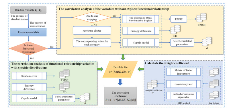
Many correlation analysis methods can capture a wide range of functional types of variables. However, the influence of uncertainty and distribution status in data is not considered, which leads to the neglect of the regularity information between variables, so that the correlation of variables that contain functional relationship but subject to specific distributions cannot be well identified. Therefore, a novel correlation analysis framework for detecting associations between variables with randomness (RVCR-CA) is proposed. The new method calculates the normalized RMSE to evaluate the degree of functional relationship between variables, calculates entropy difference to measure the degree of uncertainty in variables and constructs the copula function to evaluate the degree of dependence on random variables with distributions. Then, the weighted sum method is performed to the above three indicators to obtain the final correlation coefficient R. In the study, which considers the degree of functional relationship between variables, the uncertainty in variables and the degree of dependence on the variables containing distributions, cannot only measure the correlation of functional relationship variables with specific distributions, but also can better evaluate the correlation of variables without clear functional relationships. In experiments on the data with functional relationship between variables that contain specific distributions, UCI data and synthetic data, the results show that the proposed method has more comprehensive evaluation ability and better evaluation effect than the traditional method of correlation analysis.

| [1] | N. J. Gogtay, U. M. Thatte, Principles of correlation analysis, J. Assoc. Physicians India, 65 (2017), 78–81. |
| [2] |
J. Zhou, Y. Ma, Y. Liu, Y. Xiang, C. Cao, H. Yu, et al., A correlation analysis between the nutritional status and prognosis of COVID-19 patients, J. Nutr. Health Aging, 25 (2020), 1–10. https://doi.org/10.1007/s12603-020-1457-6 doi: 10.1007/s12603-020-1457-6

|
| [3] |
X. Xu, X. He, A. Qian, R. C. Qiu, A correlation analysis method for power systems based on random matrix theory, IEEE Trans. Smart Grid, 8 (2015), 1811–1820. https://doi.org/10.1109/tsg.2015.2508506 doi: 10.1109/tsg.2015.2508506
|
| [4] |
J. Liu, N. An, C. Ma, X. F. Li, J. Zhang, W. Zhu, et al., Correlation analysis of intestinal flora with hypertension, Exp. Ther. Med., 16 (2018), 2325–2330. https://doi.org/10.3892/etm.2018.6500 doi: 10.3892/etm.2018.6500
|
| [5] |
C. E. Shannon, A mathematical theory of communication, Bell Syst. Tech. J., 27 (1948), 584093. https://doi.org/10.1002/j.1538-7305.1948.tb01338.x doi: 10.1002/j.1538-7305.1948.tb01338.x
|
| [6] |
K. Pearson, Determination of the coefficient of correlation, Science, 30 (1909), 23–25. https://doi.org/10.1126/science.30.757.23 doi: 10.1126/science.30.757.23
|
| [7] |
V. Aguiar, I. Guedes, Shannon entropy, Fisher information and uncertainty relations for log-periodic oscillators, Physica A, 423 (2015), 72–79. https://doi.org/10.1016/j.physa.2014.12.031 doi: 10.1016/j.physa.2014.12.031
|
| [8] |
D. N. Reshef, Y. A. Reshef, H. K. Finucane, R. F. Grossman, G. McVean, P. J. Turnbaugh, et al., Detecting novel associations in large datasets, Science, 334 (2011), 1518–1524. https://doi.org/10.1126/science.1205438 doi: 10.1126/science.1205438
|
| [9] |
H. Xiong, P. Shang, Weighted multifractal cross-correlation analysis based on Shannon entropy, Commun. Nonlinear Sci. Numer. Simul., 30 (2016), 268–283. https://doi.org/10.1016/j.cnsns.2015.06.029 doi: 10.1016/j.cnsns.2015.06.029
|
| [10] |
G. J. Székely, M. L. Rizzo, N. K. Bakirov, Measuring and testing dependence by correlation of distances, Ann. Stat., 35 (2007), 2769–2794. https://doi.org/10.1214/009053607000000505 doi: 10.1214/009053607000000505
|
| [11] |
O. H. Diserud, F. Odegaard, A multiple-site similarity measure, Biol. Lett., 3 (2007), 20–22. https://doi.org/10.1098/rsbl.2006.0553 doi: 10.1098/rsbl.2006.0553
|
| [12] |
R. H. Hariri, E. M. Fredericks, K. M. Bowers, Uncertainty in big data analytics: survey, opportunities, and challenges, J. Big Data, 6 (2019), 1–16. https://doi.org/10.1186/s40537-019-0206-3 doi: 10.1186/s40537-019-0206-3
|
| [13] |
C. S. Lai, Y. Tao, F. Xu, W. W. Y. Ng, Y. W. Jia, H. L. Yuan, et al., A robust correlation analysis framework for imbalanced and dichotomous data with uncertainty, Inf. Sci., 470 (2019), 58–77. https://doi.org/10.1016/j.ins.2018.08.017 doi: 10.1016/j.ins.2018.08.017
|
| [14] |
W. G. Favieiro, A. Balbinot, Paraconsistent random forest: an alternative approach for dealing with uncertain data, IEEE Access, 7 (2019), 149714–147927. https://doi.org/10.1109/access.2019.2946256 doi: 10.1109/access.2019.2946256
|
| [15] |
X. Chen, Y. Zhu, Uncertain random linear quadratic control with multiplicative and additive noises, Asian J. Control, 23 (2020), 2849–2864. https://doi.org/10.1002/asjc.2460 doi: 10.1002/asjc.2460
|
| [16] |
Y. Yang, P. Perdikaris, Adversarial uncertainty quantification in physics-informed neural networks, J. Comput. Phys., 394 (2019), 136–152. https://doi.org/10.1016/j.jcp.2019.05.027 doi: 10.1016/j.jcp.2019.05.027
|
| [17] |
J. Ayensa-Jiménez, H. M. Doweidar, A. J. Sanz-Herrera, M. Doblaré, A new reliability-based data-driven approach for noisy experimental data with physical constraints, Comput. Methods Appl. Mech. Eng., 328 (2018), 752–774. https://doi.org/10.1016/j.cma.2017.08.027 doi: 10.1016/j.cma.2017.08.027
|
| [18] | J. P. de Villiers, K. Laskey, A. L. Jousselme, E. Blasch, A. Waal, G. Pavlin, et al., Uncertainty representation, quantification and evaluation for data and information fusion, in 2015 18th International Conference on Information Fusion (Fusion), (2015), 50–57. |
| [19] |
B. E. Niven, V. C. Deutsch, Calculating a robust correlation coefficient and quantifying its uncertainty, Comput. Geosci., 40 (2012), 1–9. https://doi.org/10.1016/j.cageo.2011.06.021 doi: 10.1016/j.cageo.2011.06.021
|
| [20] | R. A. Johnson, D. W. Wichern, Applied Multivariate Statistical Analysis, Springer Berlin, Heidelberg, (2015), 517. https://doi.org/10.1007/978-3-662-45171-7 |
| [21] | R. B. Nelsen, Concordance and copulas: a survey, in Distributions with Given Marginals and Statistical Modelling, Springer Netherlands, (2002), 167–177. https://doi.org/10.1007/978-94-017-0061-0_18 |
| [22] |
S. Kotz, Encyclopedia of statistical sciences, J. Am. Stat. Assoc., 93 (1998), 281–317. https://doi.org/10.2307/2669895 doi: 10.2307/2669895
|
| [23] | M. Jian, Discovering association with copula Entropy, preprint, arXiv: 1907.12268. |
| [24] | I. J. Schoenberg, Contributions to the problem of approximation of equidistant data by analytic functions, Part A: On the problem of smoothing or graduation, a first class of analytic approximation formulas, Quart. Appl. Math., 4 (1946), 112–141. |
| [25] | D. H. Zhang, Entropy—A measure of uncertainty of random variable, Syst. Eng. Electron., 11 (1997), 3–7. |
| [26] |
I. Farrance, R. Frenkel, Measurement uncertainty and the importance of correlation, Clin. Chem. Lab. Med., 59 (2021), 7–9. https://doi.org/10.1515/cclm-2020-1205 doi: 10.1515/cclm-2020-1205
|
| [27] | A. Sklar, Fonctions de répartition à N dimensions et leurs marges, in Annales de l'ISUP, 8 (1959), 229–231. |
| [28] | S. Ly, K. H. Pho, S. Ly, W. K. Wong, Determining distribution for the product of random variables by using copulas, Risks, 7 (2019), 23. |
| [29] |
W. E. Donath, A. J. Hoffman, Lower bounds for the partitioning of graphs, IBM J. Res. Dev., 17 (1973), 420–425. https://doi.org/10.1147/rd.175.0420 doi: 10.1147/rd.175.0420
|
| [30] |
T. L. Saaty, K. P. Kearns, The analytic hierarchy process, Anal. Plann., 1985 (1985), 19–62. https://doi.org/10.1016/b978-0-08-032599-6.50008-8 doi: 10.1016/b978-0-08-032599-6.50008-8
|
| [31] |
M. Brunelli, Introduction to the analytic hierarchy process, Springer, (2014), 33–44. https://doi.org/10.1016/B978-0-12-416727-8.00003-5 doi: 10.1016/B978-0-12-416727-8.00003-5
|
| [32] | C. D. Boor, Least squares cubic spline approximation I-fixed knots and Ⅱ-fixed knots, Purdue Univ. Rep., (1968), 10014776809. |
| [33] | D. Mukherjee, An error reduced and uniform parameter approximation in fitting of B-spline curves to data points, preprint, arXiv: 2005.08468. |
| [34] |
O. Nave, Modification of semi-analytical method applied system of ODE, Mod. Appl. Sci., 14 (2020), 75. https://doi.org/10.5539/mas.v14n6p75 doi: 10.5539/mas.v14n6p75
|
| [35] |
B. Nie, Y. W. Du, J. Q. Du, Y. Rao, Y. C. Chao, X. P. Zheng, et al., A novel regression method: Partial least distance square regression methodology, Chemom. Intell. Lab. Syst., 237 (2023), 104827. https://doi.org/10.1016/J.CHEMOLAB.2023.104827 doi: 10.1016/J.CHEMOLAB.2023.104827
|
| [36] | A. Shemyakin, A. Kniazev, Random variables and distributions, in Introduction to Bayesian Estimation and Copula Models of Dependence, John Wiley & Sons, Inc., (2017), 103–140. https://doi.org/10.1002/9781118959046.ch1 |
| [37] |
C. Genest, L. P. Rivest, Statistical inference procedures for bivariate Archimedean copulas, J. Am. Stat. Assoc., 88 (1993), 1034–1043. https://doi.org/10.1080/01621459.1993.10476372 doi: 10.1080/01621459.1993.10476372
|
| [38] |
S. Lipovetsky, Understanding the analytic hierarchy process, Technometrics, 2 (2021), 278–279. https://doi.org/10.1007/978-3-319-33861-3_2 doi: 10.1007/978-3-319-33861-3_2
|


Figures(7) / Tables(13)

Yuwen Du, Bin Nie, Jianqiang Du, Xuepeng Zheng, Haike Jin, Yuchao Zhang. New research for detecting complex associations between variables with randomness[J]. Mathematical Biosciences and Engineering, 2024, 21(1): 1356-1393. doi: 10.3934/mbe.2024059


 DownLoad: