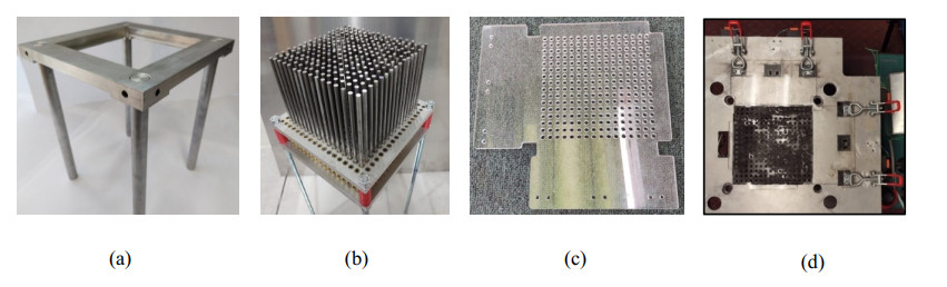
Pad printing is used in automotive, medical, electrical and other industries, employing diverse materials to transfer a 2D image onto a 3D object with different sizes and geometries. This work presents a universal fixation system for pad printing of plastic parts (UFSP4) in response to the needs of small companies that cannot afford to invest in the latest technological advances. The UFSP4 comprises two main subsystems: a mechanical support system (i.e., support structure, jig matrix and braking system) and a control system (i.e., an electronic system and an electric-hydraulic system). A relevant feature is the combination of a jig matrix and jig pins to fixate complex workpieces with different sizes. Using finite element analysis (FEA), in the mesh convergence, the total displacement converges to 0.00028781 m after 12,000 elements. The maximum equivalent stress value is 1.22 MPa for the polycarbonate plate in compliance with the safety factor. In a functionality test of the prototype performed in a production environment for one hour, the jigs fixed by the plate did not loosen, maintaining the satisfactory operation of the device. This is consistent with the displacement distribution of the creep analysis and shows the absence of the creep phenomenon. Based on FEA that underpinned the structural health computation of the braking system, the prototype was designed and built, seeking to ensure a reliable and safe device to fixate plastic parts, showing portability, low-cost maintenance and adaptability to the requirements of pad printing of automotive plastic parts.
Citation: José Alejandro Fernández Ramírez, Óscar Hernández-Uribe, Leonor Adriana Cárdenas-Robledo, Alfredo Chávez Luna. Universal fixation system for pad printing of plastic parts[J]. Mathematical Biosciences and Engineering, 2023, 20(12): 21032-21048. doi: 10.3934/mbe.2023930
Pad printing is used in automotive, medical, electrical and other industries, employing diverse materials to transfer a 2D image onto a 3D object with different sizes and geometries. This work presents a universal fixation system for pad printing of plastic parts (UFSP4) in response to the needs of small companies that cannot afford to invest in the latest technological advances. The UFSP4 comprises two main subsystems: a mechanical support system (i.e., support structure, jig matrix and braking system) and a control system (i.e., an electronic system and an electric-hydraulic system). A relevant feature is the combination of a jig matrix and jig pins to fixate complex workpieces with different sizes. Using finite element analysis (FEA), in the mesh convergence, the total displacement converges to 0.00028781 m after 12,000 elements. The maximum equivalent stress value is 1.22 MPa for the polycarbonate plate in compliance with the safety factor. In a functionality test of the prototype performed in a production environment for one hour, the jigs fixed by the plate did not loosen, maintaining the satisfactory operation of the device. This is consistent with the displacement distribution of the creep analysis and shows the absence of the creep phenomenon. Based on FEA that underpinned the structural health computation of the braking system, the prototype was designed and built, seeking to ensure a reliable and safe device to fixate plastic parts, showing portability, low-cost maintenance and adaptability to the requirements of pad printing of automotive plastic parts.

| [1] |
R. Müller, M. Vette, A. Geenen, Skill-based dynamic task allocation in human-robot-cooperation with the example of welding application, Procedia Manuf., 11 (2017), 13–21. https://doi.org/10.1016/j.promfg.2017.07.113 doi: 10.1016/j.promfg.2017.07.113

|
| [2] |
E. Olaiz, J. Zulaika, F. Veiga, M. Puerto, A. Gorrotxategi, Adaptive fixturing system for the smart and flexible positioning of large volume workpieces in the wind-power sector, Procedia CIRP, 21 (2014), 183–188. https://doi.org/10.1016/j.procir.2014.03.193 doi: 10.1016/j.procir.2014.03.193
|
| [3] | L. Joyanes, Industria 4.0: La Cuarta Revolución Industrial, 1st edition, Alfaomega Grupo Editor, 2017. |
| [4] |
V. Ivanov, F. Botko, I. Dehtiarov, M. Kočiško, A. Evtuhov, I. Pavlenko, et al., Development of flexible fixtures with incomplete locating, Machines, 10 (2022), 493. https://doi.org/10.3390/machines10070493 doi: 10.3390/machines10070493
|
| [5] | M. Jones, L. Zarzycki, G. Murray, Does industry 4.0 pose a challenge for the SME machine builder? A case study and reflection of readiness for a UK SME, in Precision Assembly in the Digital Age, Springer, (2019), 183–197. https://doi.org/10.1007/978-3-030-05931-6_17 |
| [6] |
Y. Chen, A. Klingler, K. Fu, L. Ye, 3D printing and modelling of continuous carbon fibre reinforced composite grids with enhanced shear modulus, Eng. Struct., 286 (2023), 116165. https://doi.org/10.1016/j.engstruct.2023.116165 doi: 10.1016/j.engstruct.2023.116165
|
| [7] | C. Bodenstein, H. M. Sauer, F. Fernandes, E. Dörsam, Assessing and improving edge roughness in pad-printing by using outlines in a one-step exposure process for the printing form, J. Print Media Technol. Res., 8 (2019), 19–27. |
| [8] |
T. S. S. Saikumar, Bhanumurthysoppari, C. R. Bandaru, Design and simulation of automated pad printing machine using automation studio, Mater. Today Proc., 45 (2021), 2871–2877. https://doi.org/10.1016/j.matpr.2020.11.813 doi: 10.1016/j.matpr.2020.11.813
|
| [9] |
E. Hrušková, M. Matúšová, Š. Václav, Design of construction and controlling of automation technics in order to improve skills of students, Multidiscip. Aspects Prod. Eng., 4 (2021), 120–131. https://doi.org/10.2478/mape-2021-0011 doi: 10.2478/mape-2021-0011
|
| [10] | H. Hashemi, A. M. Shaharoun, S. Izman, B. Ganji, Z. Namazian, S. Shojaei, Fixture design automation and optimization techniques: Review and future trends, Int. J. Eng. Trans. B, 27 (2014), 1787–1794. |
| [11] |
A. F. Casas Pulido, O. Bohórquez, O. A. González-Estrada, J. Quiroga, A. Pertuz, Adhesive joints for composite materials produced by additive manufacturing, J. Phys. Conf. Ser., 1386 (2019), 012005. https://doi.org/10.1088/1742-6596/1386/1/012005 doi: 10.1088/1742-6596/1386/1/012005
|
| [12] |
I. A. Daniyan, A. O. Adeodu, B. I. Oladapo, O. L. Daniyan, O. R. Ajetomobi, Development of a reconfigurable fixture for low weight machining operations, Cogent Eng., 6 (2019), 1579455. https://doi.org/10.1080/23311916.2019.1579455 doi: 10.1080/23311916.2019.1579455
|
| [13] |
A. Gameros, S. Lowth, D. Axinte, A. Nagy-Sochacki, O. Craig, H. R. Siller, State of the art in fixture systems for the manufacture and assembly of rigid components: A review, Int. J. Mach. Tools Manuf., 123 (2017), 1–21. https://doi.org/10.1016/j.ijmachtools.2017.07.004 doi: 10.1016/j.ijmachtools.2017.07.004
|
| [14] | Y. Kılıçarslan, Modular Fixture Design for CNC Machining Centers, Master thesis, Middle East Technical University in Ankara, Turkey, 2019. |
| [15] | P. Raval, N. P. Maniar, S. Thaker, P. Thanki, Industry 4.0 technology: Design and manufacturing of modular fixture, in Recent Advances in Mechanical Infrastructure, Springer, (2021), 411–417. https://doi.org/10.1007/978-981-33-4176-0_35 |
| [16] |
H. Tohidi, T. AlGeddawy, Change management in modular assembly systems to correspond to product geometry change, Int. J. Prod. Res., 57 (2019), 6048–6060. https://doi.org/10.1080/00207543.2018.1559374 doi: 10.1080/00207543.2018.1559374
|
| [17] |
A. Stornelli, S. Ozcan, C. Simms, Advanced manufacturing technology adoption and innovation: A systematic literature review on barriers, enablers, and innovation types, Res. Policy, 50 (2021), 104229. https://doi.org/10.1016/j.respol.2021.104229 doi: 10.1016/j.respol.2021.104229
|
| [18] | A. Sachdeva, R. Agrawal, C. Chaudhary, D. Siddhpuria, D. Kashyap, S. Timung, Sustainability of 3D printing in industry 4.0: A brief review, in 3D Printing Technology for Water Treatment Applications, Elsevier, (2023), 229–251. https://doi.org/10.1016/B978-0-323-99861-1.00010-2 |
| [19] |
D. R. Harish, T. Gowtham, A. Arunachalam, M. S. Narassima, D. Lamy, M. Thenarasu, Productivity improvement by application of simulation and lean approaches in an multimodel assembly line, Proc. Inst. Mech. Eng. Part B: J. Eng. Manuf., 2023. https://doi.org/10.1177/09544054231182264 doi: 10.1177/09544054231182264
|
| [20] | G. Schuh, G. Bergweiler, F. Fiedler, V. Slawik, C. Ahues, A review of data-based methods for the development of an adaptive engineering change system for automotive body shop, in Proceedings of the Conference on Production Systems and Logistics, Hannover: publish-Ing., (2021), 359–369. https://doi.org/10.15488/11295 |
| [21] |
H. Radhwan, M. S. M. Effendi, M. F. Rosli, Z. Shayfull, K. N. Nadia, Design and analysis of jigs and fixtures for manufacturing process, IOP Conf. Ser.: Mater. Sci. Eng., 551 (2019), 012028. https://doi.org/10.1088/1757-899X/551/1/012028 doi: 10.1088/1757-899X/551/1/012028
|
| [22] |
N. Ma, H. Huang, H. Murakawa, Effect of jig constraint position and pitch on welding deformation, J. Mater. Process. Technol., 221 (2015), 154–162. https://doi.org/10.1016/j.jmatprotec.2015.02.022 doi: 10.1016/j.jmatprotec.2015.02.022
|
| [23] | H. C. Pandit, Jigs and fixtures in manufacturing, Int. J. Eng. Res. Appl., 12 (2022), 50–55. |
| [24] |
S. Weckx, S. Robyns, J. Baake, E. Kikken, R. De Geest, M. Birem, et al., A cloud-based digital twin for monitoring of an adaptive clamping mechanism used for high performance composite machining, Procedia Comput. Sci., 200 (2022), 227–236. https://doi.org/10.1016/j.procs.2022.01.221 doi: 10.1016/j.procs.2022.01.221
|
| [25] |
K. Ju, C. Duan, J. Kong, Y. Chen, Y. Sun, Clamping deformation of thin circular workpiece with complex boundary in vacuum fixture system, Thin-Walled Struct., 171 (2022), 108777. https://doi.org/10.1016/j.tws.2021.108777 doi: 10.1016/j.tws.2021.108777
|
| [26] |
S. Mousavi, M. Guskov, J. Duchemin, P. Lorong, Clamping modeling in automotive flexible workpieces machining, Procedia CIRP, 101 (2021), 134–137. https://doi.org/10.1016/j.procir.2021.04.004 doi: 10.1016/j.procir.2021.04.004
|
| [27] |
H. Tohidi, T. AlGeddawy, Planning of modular fixtures in a robotic assembly system, Procedia CIRP, 41 (2016), 252–257. https://doi.org/10.1016/j.procir.2015.12.090 doi: 10.1016/j.procir.2015.12.090
|
| [28] |
M. Matejic, B. Tadic, M. Lazarevic, M. Misic, D. Vukelic, Modelling and simulation of a novel modular fixture for a flexible manufacturing system, Int. J. Simul. Model., 17 (2018), 18–29. https://doi.org/10.2507/IJSIMM17(1)407 doi: 10.2507/IJSIMM17(1)407
|
| [29] |
K. Yu, S. Wang, Y. Wang, Z. Yang, A flexible fixture design method research for similar automotive body parts of different automobiles, Adv. Mech. Eng., 10 (2018). https://doi.org/10.1177/1687814018761272 doi: 10.1177/1687814018761272
|
| [30] |
W. T. Seloane, K. Mpofu, B. I. Ramatsetse, D. Modungwa, Conceptual design of intelligent reconfigurable welding fixture for rail car manufacturing industry, Procedia CIRP, 91 (2020), 583–593. https://doi.org/10.1016/j.procir.2020.02.217 doi: 10.1016/j.procir.2020.02.217
|
| [31] |
J. Villena Toro, A. Wiberg, M. Tarkian, Application of optimized convolutional neural network to fixture layout in automotive parts, Int. J. Adv. Manuf. Technol., 126 (2023), 339–353. https://doi.org/10.1007/s00170-023-10995-0 doi: 10.1007/s00170-023-10995-0
|
| [32] |
L. Gong, H. Söderlund, L. Bogojevic, X. Chen, A. Berce, Å. Fast-Berglund, et al., Interaction design for multi-user virtual reality systems: An automotive case study, Procedia CIRP, 93 (2020), 1259–1264. https://doi.org/10.1016/j.procir.2020.04.036 doi: 10.1016/j.procir.2020.04.036
|
| [33] |
K. J. Jonsson, R. Stolt, F. Elgh, A case-based reasoning method including tooling function for case retrieval and reuse in stamping tooling design, Comput. Aided Des. Appl., 20 (2023), 839–855. https://doi.org/10.14733/cadaps.2023.839-855 doi: 10.14733/cadaps.2023.839-855
|
| [34] |
J. P. Cardona, J. J. Leal, J. U. Castellanos, J. E. Ustariz, Soluciones analíticas y numéricas de esfuerzos mecánicos en placas rectangulares isotrópicas, Inf. Tecnol., 32 (2021), 13–24. http://doi.org/10.4067/S0718-07642021000600013 doi: 10.4067/S0718-07642021000600013
|
| [35] |
L. Croppi, N. Grossi, A. Scippa, G. Campatelli, Fixture optimization in turning thin-wall components, Machines, 7 (2019), 68. https://doi.org/10.3390/machines7040068 doi: 10.3390/machines7040068
|
| [36] |
B. Zhu, Z. Mu, W. He, L. Fan, G. Zhao, Y. Yang, Research on clamping action control technology for floating fixtures, Materials, 15 (2022), 5571. https://doi.org/10.3390/ma15165571 doi: 10.3390/ma15165571
|
| [37] |
A. R. Aderiani, M. Hallmann, K. Wärmefjord, B. Schleich, R. Söderberg, S. Wartzack, Integrated tolerance and fixture layout design for compliant sheet metal assemblies, Appl. Sci., 11 (2021), 1646. https://doi.org/10.3390/app11041646 doi: 10.3390/app11041646
|
| [38] |
Y. Chen, K. Fu, B. Jiang, Modelling localised progressive failure of composite sandwich panels under in-plane compression, Thin-Walled Struct., 184 (2023), 110552. https://doi.org/10.1016/j.tws.2023.110552 doi: 10.1016/j.tws.2023.110552
|
| [39] |
M. M. Rashid, A. A. Khan, M. Usman, M. Ayub, B. Rustam, Optimization of modular fixture layout by minimizing work-piece deformation, Pak. J. Eng. Technol., 4 (2021), 43–51. https://doi.org/10.51846/vol4iss1pp43-51 doi: 10.51846/vol4iss1pp43-51
|
| [40] |
F. Veiga, T. Bhujangrao, A. Suárez, E. Aldalur, I. Goenaga, D. Gil-Hernandez, Validation of the mechanical behavior of an aeronautical fixing turret produced by a design for additive manufacturing (DfAM), Polymers, 14 (2022), 2177. https://doi.org/10.3390/polym14112177 doi: 10.3390/polym14112177
|
| [41] | Y. Xu, W. Zhang, X. Wei, B. Huang, Research on image quality control technology of pad printing, in China Academic Conference on Printing and Packaging, Springer, (2023), 163–169. https://doi.org/10.1007/978-981-19-9024-3_22 |
| [42] |
K. C. Arredondo-Soto, J. Blanco-Fernández, M. A. Miranda-Ackerman, M. M. Solís-Quinteros, A. Realyvásquez-Vargas, J. L. García-Alcaraz, A plan-do-check-act based process improvement intervention for quality improvement, IEEE Access, 9 (2021), 132779–132790. https://doi.org/10.1109/ACCESS.2021.3112948 doi: 10.1109/ACCESS.2021.3112948
|
| [43] | A. Al Aboud, E. Dörsam, D. Spiehl, Investigation of printing pad geometry by using FEM simulation, J. Print Media Technol. Res., 9 (2020), 81–93. |
| [44] |
E. Pessot, A. Zangiacomi, C. Battistella, V. Rocchi, A. Sala, M. Sacco, What matters in implementing the factory of the future: Insights from a survey in European manufacturing regions, J. Manuf. Technol. Manag., 32 (2021), 795–819. https://doi.org/10.1108/JMTM-05-2019-0169 doi: 10.1108/JMTM-05-2019-0169
|
| [45] |
T. Masood, P. Sonntag, Industry 4.0: Adoption challenges and benefits for SMEs, Comput. Ind., 121 (2020), 103261. https://doi.org/10.1016/j.compind.2020.103261 doi: 10.1016/j.compind.2020.103261
|
| [46] |
M. Sanchez, E. Exposito, J. Aguilar, Industry 4.0: Survey from a system integration perspective, Int. J. Comput. Integr. Manuf., 33 (2020), 1017–1041. https://doi.org/10.1080/0951192X.2020.1775295 doi: 10.1080/0951192X.2020.1775295
|
| [47] | S. H. Moon, Industry 4.0 for advanced manufacturing and its implementation, Eurasian J. Anal. Chem., 13 (2018), 491–497. |
| [48] |
B. Tjahjono, C. Esplugues, E. Ares, G. Pelaez, What does industry 4.0 mean to supply chain, Procedia Manuf., 13 (2017), 1175–1182. https://doi.org/10.1016/j.promfg.2017.09.191 doi: 10.1016/j.promfg.2017.09.191
|
| [49] |
X. Li, S. Yu, Y. Lei, N. Li, B. Yang, Intelligent machinery fault diagnosis with event-based camera, IEEE Trans. Ind. Inform., 2023. https://doi.org/10.1109/TII.2023.3262854 doi: 10.1109/TII.2023.3262854
|
| [50] | K. T. Ulrich, S. D. Eppinger, M. C. Yang, Product Design and Development, 7th edition, McGraw-Hill, 2019. |
| [51] | V. Balachandran, Design of Jigs, Fixtures and Press Tools, Notion Press, 2015. |
| [52] | Protel 99 SE Training Manual, PCB Design, 2001. Available from: https://www.mikrocontroller.net/attachment/17909/Protel_99_SE_Traning_Manual_PCB_Design.pdf. |
| [53] |
A. Corrado, W. Polini, Tolerance analysis tools for fixture design: A comparison, Procedia CIRP, 92 (2020), 112–117. https://doi.org/10.1016/j.procir.2020.05.174 doi: 10.1016/j.procir.2020.05.174
|
| [54] | MatWeb, Materials Information Resource, 2023. Available from: https://matweb.com/. |
| [55] |
M. Dixit, V. Mathur, S. Gupta, M. Baboo, K. Sharma, N. S. Saxena, Morphology, miscibility and mechanical properties of PMMA/PC blends, Phase Transitions, 82 (2009), 866–878. https://doi.org/10.1080/01411590903478304 doi: 10.1080/01411590903478304
|
| [56] |
Y. Chen, L. Ye, H. Dong, Lightweight 3D carbon fibre reinforced composite lattice structures of high thermal-dimensional stability, Compos. Struct., 304 (2023), 116471. https://doi.org/10.1016/j.compstruct.2022.116471 doi: 10.1016/j.compstruct.2022.116471
|
| [57] | R. C. Hibbeler, Mechanics of Materials, 11th edition, Pearson, 2022. |
| [58] |
S. Jazouli, W. Luo, F. Brémand, T. Vu-Khanh, Nonlinear creep behavior of viscoelastic polycarbonate, J. Mater. Sci., 41 (2006), 531–536. https://doi.org/10.1007/s10853-005-2276-1 doi: 10.1007/s10853-005-2276-1
|


Figures(10) / Tables(1)

José Alejandro Fernández Ramírez, Óscar Hernández-Uribe, Leonor Adriana Cárdenas-Robledo, Alfredo Chávez Luna. Universal fixation system for pad printing of plastic parts[J]. Mathematical Biosciences and Engineering, 2023, 20(12): 21032-21048. doi: 10.3934/mbe.2023930


 DownLoad: