Optimal control of a tick population with a view to control of Rocky Mountain Spotted Fever

Maeve L. McCarthy; Dorothy I. Wallace; Maeve L. McCarthy; Dorothy I. Wallace

doi:10.3934/mbe.2023837

Mathematical Biosciences and Engineering

2023, Volume 20, Issue 10: 18916-18938. doi: 10.3934/mbe.2023837

Previous Article Next Article

Research article Special Issues

Optimal control of a tick population with a view to control of Rocky Mountain Spotted Fever

Maeve L. McCarthy ^{1
,
,},
Dorothy I. Wallace ²

1.
Department of Mathematics & Statistics, Murray State University, 203A Industry & Technology, Murray KY 42071, USA
2.
Department of Mathematics, Dartmouth College, 27 N. Main Street, 6188 Kemeny Hall, Hanover, NH 03755-3551, USA

Received: 24 July 2023 Revised: 13 September 2023 Accepted: 21 September 2023 Published: 10 October 2023

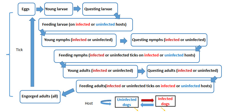
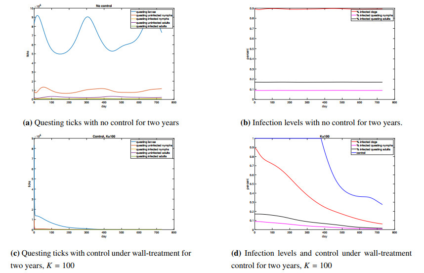
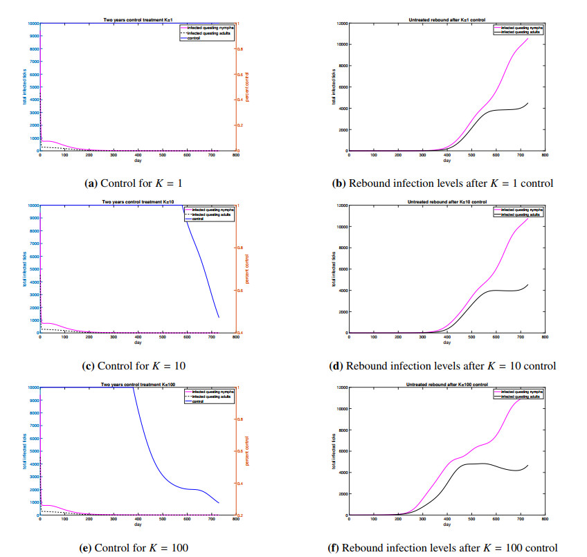
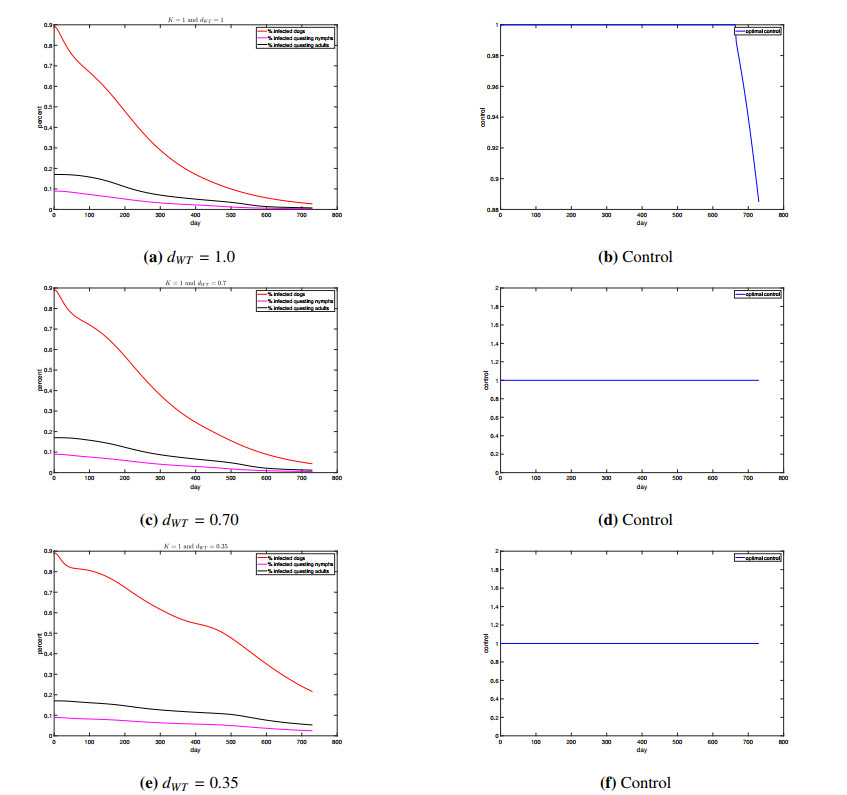
In some regions of the Americas, domestic dogs are the host for the tick vector Rhipicephalus sanguineus, and spread the tick-borne pathogen Rickettsia rickettsii, which causes Rocky Mountain Spotted Fever (RMSF) in humans. Interventions are carried out against the vector via dog collars and acaricidal wall treatments. This paper investigates the optimal control of acaricidal wall treatments, using a prior model for populations and disease transmission developed for this particular vector, host, and pathogen. It is modified with a death term during questing stages reflecting the cost of control and level of coverage. In the presence of the control, the percentage of dogs and ticks infected with Ri. rickettsii decreases in a short period and remains suppressed for a longer period, including after treatment is discontinued. Risk of RMSF infection declines by 90% during this time. In the absence of re-application, infected tick and dog populations rebound, indicating the eventual need for repeated treatment.

Keywords:

Citation: Maeve L. McCarthy, Dorothy I. Wallace. Optimal control of a tick population with a view to control of Rocky Mountain Spotted Fever[J]. Mathematical Biosciences and Engineering, 2023, 20(10): 18916-18938. doi: 10.3934/mbe.2023837

Related Papers:

[1]	Yijun Lou, Li Liu, Daozhou Gao . Modeling co-infection of Ixodes tick-borne pathogens. Mathematical Biosciences and Engineering, 2017, 14(5&6): 1301-1316. doi: 10.3934/mbe.2017067
[2]	Holly Gaff . Preliminary analysis of an agent-based model for a tick-borne disease. Mathematical Biosciences and Engineering, 2011, 8(2): 463-473. doi: 10.3934/mbe.2011.8.463
[3]	Luis Almeida, Michel Duprez, Yannick Privat, Nicolas Vauchelet . Mosquito population control strategies for fighting against arboviruses. Mathematical Biosciences and Engineering, 2019, 16(6): 6274-6297. doi: 10.3934/mbe.2019313
[4]	Mlyashimbi Helikumi, Moatlhodi Kgosimore, Dmitry Kuznetsov, Steady Mushayabasa . Dynamical and optimal control analysis of a seasonal Trypanosoma brucei rhodesiense model. Mathematical Biosciences and Engineering, 2020, 17(3): 2530-2556. doi: 10.3934/mbe.2020139
[5]	Meng Zhang, Xiaojing Wang, Jingan Cui . Sliding mode of compulsory treatment in infectious disease controlling. Mathematical Biosciences and Engineering, 2019, 16(4): 2549-2561. doi: 10.3934/mbe.2019128
[6]	Wandi Ding . Optimal control on hybrid ODE Systems with application to a tick disease model. Mathematical Biosciences and Engineering, 2007, 4(4): 633-659. doi: 10.3934/mbe.2007.4.633
[7]	Yunfeng Liu, Guowei Sun, Lin Wang, Zhiming Guo . Establishing Wolbachia in the wild mosquito population: The effects of wind and critical patch size. Mathematical Biosciences and Engineering, 2019, 16(5): 4399-4414. doi: 10.3934/mbe.2019219
[8]	Marco Tosato, Xue Zhang, Jianhong Wu . A patchy model for tick population dynamics with patch-specific developmental delays. Mathematical Biosciences and Engineering, 2022, 19(5): 5329-5360. doi: 10.3934/mbe.2022250
[9]	Rinaldo M. Colombo, Mauro Garavello . Optimizing vaccination strategies in an age structured SIR model. Mathematical Biosciences and Engineering, 2020, 17(2): 1074-1089. doi: 10.3934/mbe.2020057
[10]	Bevina D. Handari, Dipo Aldila, Bunga O. Dewi, Hanna Rosuliyana, Sarbaz H. A. Khosnaw . Analysis of yellow fever prevention strategy from the perspective of mathematical model and cost-effectiveness analysis. Mathematical Biosciences and Engineering, 2022, 19(2): 1786-1824. doi: 10.3934/mbe.2022084

Abstract

1. Introduction

Several species of ticks specialize as parasites of domestic dogs, including both temperate and tropical Rhipicephalus species ^[1]. In the U.S., Rhipicephalus sanguineus carries multiple pathogens of veterinary importance as well as Rickettsia rickettsii, the species that causes Rocky Mountain Spotted fever (RMSF) in humans ^[2,3,4,5,6].

Rocky Mountain Spotted fever is caused by one of several Rickettsia species which, together, comprise multiple pathogens, have worldwide distribution, and are carried by several vector species ^[7,8,9]. The resulting diseases range from mild to, in the case of RMSF, fatal ^[10,11].

Rhipicephalus sanguineus maturation times and death rates are dependent on temperature and humidity ^[12,13]. Thus it is not surprising that climate has been offered as an explanation of the expansion of ticks and tick-borne disease northwards ^[14,15]. Both temperate and tropical lineages of Rh. sanguineus have been identified in the U.S. ^{[16,17,18,19]}. Additionally, the incidence of RMSF has increased in the the U.S. ^{[20,21,22,23,24]}.

In general, vector borne pathogens cause a large burden of disease and mortality worldwide, and are principally controlled by vector suppression, either alone or as part of a holistic approach that may include wall treatments, dog collars or other interventions ^[25,26,27]. As vector control carries a cost as well as benefits, it is possible to approach the questions of how much and when to apply interventions via the use of optimal control methods ^[28,29]. This approach requires a system of differential equations describing the life cycle of Rh. sanguineus and disease transmission of Ri. rickettsii. Such a model was developed for populations of ticks and dogs in a community in Sonora, Mexico, and is used as the basis for the control problem solved for that model ^[30,31]. The population/transmission model takes into account the multiple stages in tick development, including temperature and humidity dependence ^[12,32]. It incorporates insecticidal wall treatment and the resulting death rate for questing ticks.

In the Sonora intervention, a small number of houses were treated with insecticidal wall treatments ^[31]. The model created for this intervention indicated that it was likely that sufficient wall coverage would remove the need for the primary intervention in that situation, which was treated dog collars ^[30]. Wall treatments in general have a short half-life, requiring re-application. Without re-application it is possible to compare limitations of treatment using models, as was done in the case of malaria. In this study we omit decay of the treatment and instead use an optimal control approach to ask how long and at what level of effectiveness the treatment must remain in place to suppress the vector population.

2. Materials & methods

The numerical approach includes a system of ordinary differential equations describing the life cycle of Rh. sanguineus, dog population growth and transmission of Ri. rickettsii between these, shown in equations (2.1-refhumidity). The control problem is framed by a system of ordinary differential equations for the adjoint variables, in equations (2.44-2.69). Results of numerical simulations are shown in Figures 2-4.

2.1. Model details

The process based model for Rh. sanguineus life cycle and disease transmission, on which optimal control is based, is taken from Álvarez-Hernandez et al, parameterized to reflect local conditions in a town in Sonora, Mexico ^[30]. The default death rate due to treatment is set at 0.7 to reflect 70% coverage of walls. That model includes temperature dependent maturation rates for non-questing stages as well as a temperature and humidity dependent death rate for questing nymphs. A condensed version of the compartment model is illustrated in Figure 1. Like other hard-bodied ticks, Rh. sanguineus passes through maturation stages (larva, nymph, adult). These stages conclude with relatively short questing (searching for a host) and feeding intervals that provide all the needed food and water for the tick to complete its lifecycle, after which it ovipositions (if female) and dies ^[32]. During the relatively long intervals between feeding on a host and the next questing event, these ticks sequester in cracks in walls, floors, and other peri-domestic areas, making them difficult to observe. Parameters are therefore adjusted to match data for questing and feeding ticks.

Figure 1. Diagram of life cycle and infection status of R. sanguineus and dog hosts. Cross transmission occurs between dogs and feeding nymphs and adults. Transmission arrows are omitted for clarity.

DownLoad: Full-Size Img PowerPoint

During the feeding stages disease transmission can take place from an infected tick to an uninfected dog, or from an infected dog to an uninfected tick. The disease transmission model is based on the Ross-Macdonald model for mosquito borne disease, with the additional feature that transmission may occur during any of the three feeding stages of the vector. There is evidence that vertical transmission may also occur, as it does in closely related diseases ^[33,34,35]. Little, however, is known about the rates involved or whether it is indeed a characteristic of this particular vector/disease pair, so this aspect of transmission is omitted from the model.

2.1.1. Differential equations for Population Dynamics & Disease Transmission

Eggs, $E$

$\begin{equation} \frac{dE}{dt} = b A_5 - m_e (metemp) E-d_e E, \end{equation}$

(2.1)

Young, hardening larvae, $L_1$

$\begin{equation} \frac{dL_1}{dt} = m_e (metemp) E - d_{UL} L_1 - m_1 L_1, \end{equation}$

(2.2)

Questing larvae, $L_2$

$\begin{equation} \frac{dL_2}{dt} = m_1 L_1 - d_{UL} L_2 - m_2 L_2 -wd_{WT} L_2, \end{equation}$

(2.3)

Larvae feeding on uninfected host, $L_U$

$\begin{equation} \frac{dL_U}{dt} = m_2 L_2 F_d Q_d -d_3 L_U -m_{3} L_U; \end{equation}$

(2.4)

Larvae feeding on infected host, $L_I$

$\begin{equation} \frac{dL_I}{dt} = m_2 L_2 F_f Q_f -d_3 dL_I-m_{3f} dL_I , \end{equation}$

(2.5)

Uninfected engorged maturing larvae/young nymphs, $NU_1$

$\begin{equation} \frac{dNU_1}{dt} = m_{3d} L_U +(1-p_L) ( m_{3f} L_I) - d_{L} NU_1-m_L (m3temp) NU_1, \end{equation}$

(2.6)

Infected engorged maturing larvae/young nymphs, $NI_1$

$\begin{equation} \frac{dNI_1}{dt} = p_L (m_{3f} L_I)- d_{L} NI_1- m_L (m3temp) NI_1, \end{equation}$

(2.7)

Questing uninfected nymphs, $NU_2$

$\begin{equation} \frac{dNU_2}{dt} = m_L(m3temp) NU_1 - d_{UN} NU_2 -m_{n2} NU_2 - w d_{WT} NU_2 , \end{equation}$

(2.8)

Questing infected nymphs, $NI_2$

$\begin{equation} \frac{dNI_2}{dt} = m_L (m3temp) NI_1-d_{UN} NI_2-m_{n2} NI_2 - w d_{WT} NI_2 , \end{equation}$

(2.9)

Uninfected nymphs feeding on uninfected hosts, $FNU_U$

$\begin{equation} \frac{dFNU_U}{dt} = m_{n2} NU_2 G_d Q_d-d_{fn} FNU_U-m_{fn} FNU_U, \end{equation}$

(2.10)

Uninfected nymphs feeding on infected hosts, $FNU_I$

$\begin{equation} \frac{dFNU_I}{dt} = m_{n2} NU_2 G_f Q_f- d_{fn} FNU_I -m_{fn} FNU_I, \end{equation}$

(2.11)

Infected nymphs feeding on uninfected hosts, $FNI_U$

$\begin{equation} \frac{dFNI_U}{dt} = m_{n2} NI_2 G_d Q_d-d_{fn} FNI_U-m_{fn} FNI_U, \end{equation}$

(2.12)

Infected nymphs feeding on Infected hosts, $FNI_I$

$\begin{equation} \frac{dFNI_I}{dt} = m_{n2} NI_2 G_f Q_f-d_{fn} FNI_I-m_{fn} FNI_I, \end{equation}$

(2.13)

Uninfected engorged maturing nymphs/young adults, $AU_1$

$\begin{equation} \frac{dAU_1}{dt} = m_{fn} (FNU_U)+m_{fn} (1-p_N)*(FNU_I)-f_{ND} AU_1- (mfntemp) AU_1, \end{equation}$

(2.14)

Infected engorged maturing nymphs/young adults, $AI_1$

$\begin{equation} \frac{dAI_1}{dt} = m_{fn} (FNI_I)+ m_{fn} FNI_I +m_{fn} (p_N) (FNU_I)-f_{ND} AI_1- (mfntemp) AI_1, \end{equation}$

(2.15)

Questing uninfected adult, $AU_2$

$\begin{equation} \frac{dAU_2}{dt} = (mfntemp) AU_1-d_{UA} AU_2-m_{A2} AU_2 - w d_{WT}AU_2, \end{equation}$

(2.16)

Questing infected adult, $AI_2$

$\begin{equation} \frac{dAI_2}{dt} = (mfntemp) AI_1-d_{UA} AI_2-m_{A2} AI_2 - wd_{WT}AI_2, \end{equation}$

(2.17)

Uninfected adults feeding on uninfected hosts, $FAU_U$

$\begin{equation} \frac{dFAU_U}{dt} = m_{A2} AU_2 H_d*Q_d- d_{A3} FAU_U- m_{A3} FAU_, \end{equation}$

(2.18)

Uninfected adults feeding on infected hosts, $FAU_I$

$\begin{equation} \frac{dFAU_I}{dt} = m_{A2} AU_2 H_f Q_f-d_{A3} FAU_I-m_{A3} FAU_I, \end{equation}$

(2.19)

Infected adults feeding on uninfected hosts, $FAI_U$

$\begin{equation} \frac{dFAI_U}{dt} = m_{A2} AI_2 H_d Q_d- d_{A3} FAI_U-m_{A3} FAI_U, \end{equation}$

(2.20)

Infected adults feeding on infected hosts, $FAI_I$

$\begin{equation} \frac{dFAI_I}{dt} = m_{A2} AI_2 H_f Q_f- d_{A3} FAI_I-m_{A3} FAI_I, \end{equation}$

(2.21)

Engorged adults, $A_4$

$\begin{equation} \frac{dA_4}{dt} = m_{A3}*(FAU_U+FAU_I + FAI_U+FAI_I)- (mfntemp) A_4, \end{equation}$

(2.22)

Gestating adults, $A_5$

$\begin{equation} \frac{dA_5}{dt} = (mfntemp) A_4 - d_{A5}*A_5, \end{equation}$

(2.23)

Uninfected hosts (dogs), $U$

$\begin{equation} \frac{dU}{dt} = b_H (U+I) (1-(U+I)/K_H)-d_H U-J_H, \end{equation}$

(2.24)

Infected hosts (dogs), $I$

$\begin{equation} \frac{dI}{dt} = J_H -d_{HI} I, \end{equation}$

(2.25)

2.1.2. Auxiliary equations

All nymphs and adults feeding on uninfected hosts, $T_U$

$\begin{equation} T_U = FNU_U+FNI_U+ FAU_U+ FAI_U, \end{equation}$

(2.26)

All nymphs and adults feeding on infected hosts

$\begin{equation} T_I = FNU_I+FNI_I+ FAU_I+ FAI_I \end{equation}$

(2.27)

Percent available space per uninfected host weighted by probability ( $q_L$ ) of larvae finding any host, $F_d$

$\begin{equation} F_d = max(q_L (C U-T_U)/(C U + \epsilon), 0), \end{equation}$

(2.28)

Percent available space per infected host weighted by probability ( $q_L$ ) of larvae finding any host, $F_f$

$\begin{equation} F_f = max(q_L (C I-T_I)/(C I + \epsilon), 0), \end{equation}$

(2.29)

Percent available space per uninfected host weighted by probability ( $q_N$ ) of nymph finding any host, $G_d$

$\begin{equation} Gd = max(q_N (C U-T_U)/(C U + \epsilon), 0), \end{equation}$

(2.30)

Percent available space per infected host weighted by probability ( $q_N$ ) of nymph finding any host, $G_f$

$\begin{equation} Gf = max(q_N (C I-T_I)/(C I + \epsilon), 0), \end{equation}$

(2.31)

Percent available space per uninfected host weighted by probability ( $q_A$ ) of adult finding any host, $H_d$

$\begin{equation} Hd = max(q_A (C U-T_U)/(C U + \epsilon), 0), \end{equation}$

(2.32)

Percent available space per infected host weighted by probability ( $q_A$ ) of adult finding any host, $H_f$

$\begin{equation} Hf = max(q_A (C I-T_I)/(C I + \epsilon), 0), \end{equation}$

(2.33)

Total number of hosts of all types, $S$

$\begin{equation} S = U+ I, \end{equation}$

(2.34)

Fraction of hosts that are uninfected, $Q_d$

$\begin{equation} Qd = U/(S+P3d), \end{equation}$

(2.35)

Fraction of hosts that are infected, $Q_f$

$\begin{equation} Qf = I/(S+P3f), \end{equation}$

(2.36)

Transmission term for host infection, $J$

$\begin{equation} J = p_{UI} (FNI_U+FAI_U) U, \end{equation}$

(2.37)

Temperature approximation for study area, $T$

$\begin{eqnarray} T = 24.84 + -8.501*cos(t*0.01721) + -1.668*sin(t*0.01721) + \end{eqnarray}$

(2.38)

$\begin{eqnarray} -0.08626*cos(2*t*0.01721) + 1.192*sin(2*t*0.01677), \end{eqnarray}$

(2.39)

Percent humidity approximation for study area, $H$

$\begin{eqnarray} H = 62.93 + 9.866*cos(t*0.01721) + -10.86*sin(t*0.01721) + \end{eqnarray}$

(2.40)

$\begin{eqnarray} 3.166*cos(2*t*0.01721) + 0.6116*sin(2*t*0.01721), \end{eqnarray}$

(2.41)

2.1.3. Properties of the Population Dynamics & Disease Transmission Model

In this section we will obtain the existence, uniqueness, nonnegativity, and boundedness of solutions to our model in a single theorem.

Theorem 2.1. For nonnegative initial conditions, the model (2.1-2.25) has a unique solution which exists for all time and is nonnegative in each component.

Proof: Local existence and uniqueness is standard via arguments in ^[36]. A supersolution argument establishes that the solutions are bounded on their interval of existence ^[37]. A subsolution argument proves that the solutions are bounded below by zero.

2.2. Optimal control

We wish to minimize the tick population during the questing life stages, $L_2, NU_2, NI_2, AU_2$ and $AI_2,$ while also minimizing the death rate caused by the wall treatment intervention, represented by the coefficient $w$ in equations (2.3, 2.8, 2.9, 2.16, 2.17).

$\begin{equation} J(w) = \min\limits_{w(t)} \int_0^T \left( L_2^2(t) + NU_2^2(t) +NI_2^2(t) +AU_2^2(t) + AI_2^2(t) + Kw^2(t) \right) \, dt \end{equation}$

(2.42)

over the set of admissible controls

$\begin{equation} V = \left\{w \text{ measurable } | \quad 0\leq w(t) \leq 1, \forall t \in [0, T] \right\}. \end{equation}$

(2.43)

We use quadratic terms in the cost function, $J(w)$ , as is typical for epidemiology control problems, because linear control does not offer closed-form solutions for the optimal control ^{[38,39,40,41]}. Often a linear-quadratic cost function is used as well. These cost functions represent the nonlinear increase in the effect of each quantity in $J(w)$ . The cost of increased infective ticks is probably closer to quadratic than linear because at low levels ticks would prefer the dog host, while at high levels they might prefer humans as space on dogs becomes saturated. Similarly, the effects of the wall treatment probably represent a nonlinear function to the system because after the more willing participants have treated their walls it becomes increasingly expensive to convince the holdouts.

The quadratic term is multiplied by a coefficient, $K$ , which allows for the relative importance of the term to be varied. The final time $T$ determines the size of the interval of existence for the optimal control.

2.3. Existence of optimal control

Theorem 2.2. Given the objective functional (2.42), subject to the system given by Eqs. (2.1-2.25) with nonnegative initial conditions, and the admissible control set (2.43) then there exists an optimal control $w^*(t)$ such that

$\min\limits_{w\in V} J(w) = J(w^*).$

Proof: In order to apply the theory of Fleming and Rishel, ^[42], we must show that the following conditions are met:

1. The class of all initial conditions with a control fnction $w(t)$ in the admissible control set along with each state equation being satisfied is not empty.

2. The admissible control set $V$ is closed and convex.

3. Each right hand side of the state system is continuous, is bounded above by a sum of the bounded control and the state, and can be written as a linear function of the control function $w(t)$ with coefficients depending on time and the state.

4. The integrand of the objective functional (2.42) is convex on $V$ and is bounded below.

Since all conditions are satisfied in this case, it follows that there exists an optimal control $w^*(t)$ such that

$\min\limits_{w\in V} J(w) = J(w^*).$

2.3.1. Characterization of Optimal Control

Theorem 2.3. Given the optimal controls $w^*$ and solutions of the corresponding state system, there exist adjoint variables $\lambda_1, \lambda_2, \ldots, \lambda_{25}$ satisfying the following:

$\begin{eqnarray} \frac{d\lambda_1}{dt} & = & \lambda_1(m_e (metemp)+d_e) -\lambda_2m_e(metemp) \end{eqnarray}$

(2.44)

$\begin{eqnarray} \frac{d\lambda_2}{dt} & = & \lambda_2(d_w+m_1) -\lambda_3m_1 \end{eqnarray}$

(2.45)

$\begin{eqnarray} \frac{d\lambda_3}{dt} & = & - 1 +\lambda_3(d_w+m_2+wd_{WT}) -\lambda_4m_2F_dQ_d - \lambda_5m_2F_fQ_f \end{eqnarray}$

(2.46)

$\begin{eqnarray} \frac{d\lambda_4}{dt} & = & \lambda_4(d_3+m_{3d}) -\lambda_6m_{3d} \end{eqnarray}$

(2.47)

$\begin{eqnarray} \frac{d\lambda_5}{dt} & = & \lambda_5(d_3+m_{3f}) -\lambda_6(1-p_L)m_{3f} +\lambda_7p_Lm_{3f} \end{eqnarray}$

(2.48)

$\begin{eqnarray} \frac{d\lambda_6}{dt} & = & \lambda_6(d_L+m_L(m3temp)) -\lambda_8m_L(m3temp) \end{eqnarray}$

(2.49)

$\begin{eqnarray} \frac{d\lambda_7}{dt} & = & \lambda_7(d_L+m_L(m3temp)) -\lambda_9m_L(m3temp) \end{eqnarray}$

(2.50)

$\begin{eqnarray} \frac{d\lambda_8}{dt} & = & - 1 +\lambda_8(d_{UN}+m_{n2}+wd_{WT}) -\lambda_{10}m_{n2}G_dQ_d - \lambda_{11}m_{n2}G_fQ_f \end{eqnarray}$

(2.51)

$\begin{eqnarray} \frac{d\lambda_9}{dt} & = & - 1 +\lambda_9(d_{UN}+m_{n2}+wd_{WT}) -\lambda_{12}m_{n2}G_dQ_d - \lambda_{13}m_{n2}G_fQ_f \end{eqnarray}$

(2.52)

$\begin{eqnarray} \frac{d\lambda_{10}}{dt} & = & \lambda_{10}(d_{fn}+m_{fn}) -\lambda_{14}m_{fn} - \lambda_4m_2L_2 \frac{\partial F_d}{\partial FNU_U} Q_d \\ &&-\lambda_{10}m_{n2}NU_2 \frac{\partial G_d}{\partial FNU_U} Q_d -\lambda_{12}m_{n2}NI_2 \frac{\partial G_d}{\partial FNU_U} Q_d \\ && -\lambda_{18}m_{A2}AU_2 \frac{\partial H_d}{\partial FNU_U} Q_d -\lambda_{20}m_{A2}AI_2 \frac{\partial H_d}{\partial FNU_U} Q_d \end{eqnarray}$

(2.53)

$\begin{eqnarray} \frac{d\lambda_{11}}{dt} & = & \lambda_{11}(d_{fn}+m_{fn}) -\lambda_{14}m_{fn}(1-p_N) -\lambda_{15}m_{fn}p_N \\ && - \lambda_5m_2L_2 \frac{\partial F_f}{\partial FNU_I} Q_f -\lambda_{11}m_{n2}NU_2 \frac{\partial G_f}{\partial FNU_I} Q_f -\lambda_{13}m_{n2}NI_2 \frac{\partial G_f}{\partial FNU_I} Q_f \\ && -\lambda_{19}m_{A2}AU_2 \frac{\partial H_f}{\partial FNU_I} Q_f -\lambda_{21}m_{A2}AI_2 \frac{\partial H_f}{\partial FNU_I} Q_f \end{eqnarray}$

(2.54)

$\begin{eqnarray} \frac{d\lambda_{12}}{dt} & = & \lambda_{12}(d_{fn}+m_{fn}) -\lambda_{25}p_{UI}U - \lambda_4m_2L_2 \frac{\partial F_d}{\partial FNI_U} Q_d \\ &&-\lambda_{10}m_{n2}NU_2 \frac{\partial G_d}{\partial FNI_U} Q_d -\lambda_{12}m_{n2}NI_2 \frac{\partial G_d}{\partial FNI_U} Q_d \\ && -\lambda_{18}m_{A2}AU_2 \frac{\partial H_d}{\partial FNI_U} Q_d -\lambda_{20}m_{A2}AI_2 \frac{\partial H_d}{\partial FNI_U} Q_d \end{eqnarray}$

(2.55)

$\begin{eqnarray} \frac{d\lambda_{13}}{dt} & = & \lambda_{13}(d_{fn}+m_{fn}) -\lambda_{15}m_{fn} \\ && - \lambda_5m_2L_2 \frac{\partial F_f}{\partial FNI_I} Q_f -\lambda_{11}m_{n2}NU_2 \frac{\partial G_f}{\partial FNI_I} Q_f -\lambda_{13}m_{n2}NI_2 \frac{\partial G_f}{\partial FNI_I} Q_f \\ && -\lambda_{19}m_{A2}AU_2 \frac{\partial H_f}{\partial FNI_I} Q_f -\lambda_{21}m_{A2}AI_2 \frac{\partial H_f}{\partial FNI_I} Q_f \end{eqnarray}$

(2.56)

$\begin{eqnarray} \frac{\lambda_{14}}{dt} & = & \lambda_{14}(f_{ND}+(mfntemp)+d_{WT}) + \lambda_{16}(mfntemp) \end{eqnarray}$

(2.57)

$\begin{eqnarray} \frac{\lambda_{15}}{dt} & = & \lambda_{15}(f_{ND}+(mfntemp)) + \lambda_{17}(mfntemp) \end{eqnarray}$

(2.58)

$\begin{eqnarray} \frac{\lambda_{16}}{dt} & = & -1+\lambda_{16}(d_{UA}+m_{A2}+wd_{WT}) - \lambda_{18}m_{A2}H_dQ_d -\lambda_{19}m_{A2}H_fQ_f \end{eqnarray}$

(2.59)

$\begin{eqnarray} \frac{\lambda_{17}}{dt} & = & -1+\lambda_{17}(d_{UA}+m_{A2}+wd_{WT}) - \lambda_{20}m_{A2}H_dQ_d -\lambda_{21}m_{A2}H_fQ_f \end{eqnarray}$

(2.60)

$\begin{eqnarray} \frac{d\lambda_{18}}{dt} & = & \lambda_{18}(d_{A3}+m_{A3}) -\lambda_{22}m_{A3} - \lambda_4m_2L_2 \frac{\partial F_d}{\partial FAU_U} Q_d \\ &&-\lambda_{10}m_{n2}NU_2 \frac{\partial G_d}{\partial FAU_U} Q_d -\lambda_{12}m_{n2}NI_2 \frac{\partial G_d}{\partial FAU_U} Q_d \\ && -\lambda_{18}m_{A2}AU_2 \frac{\partial H_d}{\partial FAU_U} Q_d -\lambda_{20}m_{A2}AI_2 \frac{\partial H_d}{\partial FAU_U} Q_d \end{eqnarray}$

(2.61)

$\begin{eqnarray} \frac{d\lambda_{19}}{dt} & = & \lambda_{19}(d_{A3}+m_{A3}) -\lambda_{22}m_{A3} \\ && - \lambda_5m_2L_2 \frac{\partial F_f}{\partial FAU_I} Q_f -\lambda_{11}m_{n2}NU_2 \frac{\partial G_f}{\partial FAU_I} Q_f -\lambda_{13}m_{n2}NI_2 \frac{\partial G_f}{\partial FAU_UI} Q_f \\ && -\lambda_{19}m_{A2}AU_2 \frac{\partial H_f}{\partial FAU_I} Q_f -\lambda_{21}m_{A2}AI_2 \frac{\partial H_f}{\partial FAU_I} Q_f \end{eqnarray}$

(2.62)

$\begin{eqnarray} \frac{d\lambda_{20}}{dt} & = & \lambda_{20}(d_{A3}+m_{A3}) -\lambda_{22}m_{A3} -\lambda_{25}p_{UI}U - \lambda_4m_2L_2 \frac{\partial F_d}{\partial FAI_U} Q_d \\ &&-\lambda_{10}m_{n2}NU_2 \frac{\partial G_d}{\partial FAI_U} Q_d -\lambda_{12}m_{n2}NI_2 \frac{\partial G_d}{\partial FAI_U} Q_d \\ && -\lambda_{18}m_{A2}AU_2 \frac{\partial H_d}{\partial FAI_U} Q_d -\lambda_{20}m_{A2}AI_2 \frac{\partial H_d}{\partial FAI_U} Q_d \end{eqnarray}$

(2.63)

$\begin{eqnarray} \frac{d\lambda_{21}}{dt} & = & \lambda_{21}(d_{A3}+m_{A3}) -\lambda_{22}m_{A3} \\ && - \lambda_5m_2L_2 \frac{\partial F_f}{\partial FAI_I} Q_f -\lambda_{11}m_{n2}NU_2 \frac{\partial G_f}{\partial FAI_I} Q_f -\lambda_{13}m_{n2}NI_2 \frac{\partial G_f}{\partial FAI_UI} Q_f \\ && -\lambda_{19}m_{A2}AU_2 \frac{\partial H_f}{\partial FAI_I} Q_f -\lambda_{21}m_{A2}AI_2 \frac{\partial H_f}{\partial FAI_I} Q_f \end{eqnarray}$

(2.64)

$\begin{eqnarray} \frac{d\lambda_{22}}{dt} & = & \lambda_{22} (mfntemp) -\lambda_{23}(mfntemp) \end{eqnarray}$

(2.65)

$\begin{eqnarray} \frac{d\lambda_{23}}{dt} & = & - \lambda_1 b + \lambda_{23} (d_{A5}) \end{eqnarray}$

(2.66)

$\begin{eqnarray} \frac{d\lambda_{24}}{dt} & = & -\lambda_4m_2L_2\left( \frac{\partial F_d}{\partial U} Q_d +F_d\frac{\partial Q_d}{\partial U} \right) -\lambda_5m_2L_2F_f\frac{\partial Q_f}{\partial U} \\ && -\lambda_{10}m_{n2}NU_2\left( \frac{\partial G_d}{\partial U} Q_d +G_d\frac{\partial Q_d}{\partial U} \right) -\lambda_{11}m_{n2}NU_2G_f\frac{\partial Q_f}{\partial U} \\ &&-\lambda_{12}m_{n2}NI_2\left( \frac{\partial G_d}{\partial U} Q_d +G_d\frac{\partial Q_d}{\partial U} \right) -\lambda_{13}m_{n2}NI_2G_f\frac{\partial Q_f}{\partial U} \\ && -\lambda_{18}m_{A2}AU_2\left( \frac{\partial H_d}{\partial U} Q_d +H_d\frac{\partial Q_d}{\partial U} \right) -\lambda_{19}m_{A2}AU_2H_f\frac{\partial Q_f}{\partial U} \\ && -\lambda_{20}m_{A2}AI_2\left( \frac{\partial H_d}{\partial U} Q_d +H_d\frac{\partial Q_d}{\partial U} \right) -\lambda_{21}m_{A2}AI_2H_f\frac{\partial Q_f}{\partial U} \\ && -\lambda_{24}\left( b_H\left(1- \frac{2(U+I)}{K_H}\right) -d_H\right) -\lambda_{25}p_{UI}(FNI_U+FAI_U) \end{eqnarray}$

(2.67)

$\begin{eqnarray} \frac{d\lambda_{25}}{dt} & = & -\lambda_4m_2L_2F_d\frac{\partial Q_d}{\partial I} -\lambda_5m_2L_2\left(\frac{\partial F_f}{\partial I} Q_f+ F_f\frac{\partial Q_f}{\partial I}\right) \\ && -\lambda_{10}m_{n2}NU_2G_d \frac{\partial Q_d}{\partial I} -\lambda_{11}m_{n2}NU_2\left(\frac{\partial G_f}{\partial I} Q_f+ G_f\frac{\partial Q_f}{\partial I} \right) \\ && -\lambda_{12}m_{n2}NI_2G_d \frac{\partial Q_d}{\partial I} -\lambda_{13}m_{n2}NI_2\left(\frac{\partial G_f}{\partial I} Q_f+ G_f\frac{\partial Q_f}{\partial I} \right) \\ && -\lambda_{18}m_{A2}AU_2H_d \frac{\partial Q_d}{\partial I} -\lambda_{19}m_{A2}AU_2\left(\frac{\partial H_f}{\partial I} Q_f+ H_f\frac{\partial Q_f}{\partial I} \right) \\ && -\lambda_{20}m_{A2}AI_2H_d \frac{\partial Q_d}{\partial I} -\lambda_{21}m_{A2}AI_2\left(\frac{\partial H_f}{\partial I} Q_f+ H_f\frac{\partial Q_f}{\partial I} \right) \\ && -\lambda_{24}b_H\left(1- \frac{2(U+I)}{K_H}\right) -\lambda_{25}d_{HI} \end{eqnarray}$

(2.68)

where $\lambda_1(T) = \lambda_2(T) = \cdots = \lambda_{25}(T) = 0.$ Furthermore, the analytic representation of the optimal control $w^*$ is given by

$\begin{equation} w^*(t) = \min\left( \max\left(0, \frac{\left(\lambda_3 L_2+\lambda_8 NU_2 +\lambda_9 NI_2 +\lambda_{16} AU_2 +\lambda_{17}AI_2 \right) d_{WT}}{2K} \right), 1 \right) \end{equation}$

(2.69)

Note that

$\frac{\partial F_d}{\partial U} = \left\{\begin{array}{ll} q_L \left(\frac{C(T_U+\epsilon)}{(CU+\epsilon)^2}\right) & \mbox{if } CU-T_U > 0 \\ 0 & \mbox{otherwise} \end{array} \right.$

and

$\frac{\partial F_d}{\partial FNU_U} = \frac{\partial F_d}{\partial FNI_U} = \frac{\partial F_d}{\partial FAU_U} = \frac{\partial F_d}{\partial FAI_U} = \left\{\begin{array}{ll} \frac{-q_L}{CU+\epsilon} & \mbox{if } CU-T_U > 0 \\ 0 & \mbox{otherwise} \end{array} \right.$

and

$\frac{\partial F_f}{\partial I} = \left\{\begin{array}{ll} q_L \left(\frac{C(T_I+\epsilon)}{(CI+\epsilon)^2}\right) & \mbox{if } CI-T_I > 0 \\ 0 & \mbox{otherwise} \end{array} \right.$

and

$\frac{\partial F_f}{\partial FNU_I} = \frac{\partial F_f}{\partial FNI_I} = \frac{\partial F_f}{\partial FAU_I} = \frac{\partial F_d}{\partial FAI_I} = \left\{\begin{array}{ll} \frac{-q_L}{CI+\epsilon} & \mbox{if } CI-T_I > 0 \\ 0 & \mbox{otherwise} \end{array} \right.$

with similar expressions for $G_d, G_f, H_d, H_f.$

Proof: Suppose $w^*(t)$ is the optimal control and that $E, {\rm{Ł}}_1, \ldots, U, I$ is the corresponding solution to the system (2.1-2.25). We use standard work in Pontryagin et al. ^[32] to obtain the result. To find the analytic representation of the optimal control $w^*(t),$ begin by forming the Lagrangian. Since the control is bounded, the Lagrangian is

$\mathcal{L} = H-W_1(t)\left( w(t) -0\right) - W_2(t)\left( 1-w(t) \right)$

where H is the Hamiltonian given by

$H = L_2+NU_2+NI_2+AU_2+AI_2+Kw^2 + \sum\limits_{i = 1}^{25} \lambda_i \left( rhs_i\right)$

and $W_i(t) \geq 0$ are penalty multipliers such that

$\left. \begin{array}{l} W_1(t) (w(t) -0) = 0\\ W_2(t) (1-w(t)) = 0 \end{array} \right\} \mbox{at } w^*(t)$

To find the analytic representation for $w^*(t),$ we analyze the necessary conditions for optimality $\frac{\partial\mathcal{L}}{\partial w} = 0.$

$\frac{\partial\mathcal{L}}{\partial w} = \frac{\partial H}{\partial w} -W_1+W_2 = 0$

$2Kw + \lambda_3(-d_{WT}L_2) + \lambda_8 (-d_{WT}NU_2) + \lambda_9(-d_{WT}NI_2) +\lambda_{16}(d_{WT}AU_2 + \lambda_{17}(-d_{WT}AI_2) - W1+W2 = 0.$

By standard optimality techniques for the characterization for the optimal control $w^*(t)$ , we find that

$w^*(t) = \min\left( \max\left(0, \frac{\left(\lambda_3 L_2+\lambda_8 NU_2 +\lambda_9 NI_2 +\lambda_{16} AU_2 +\lambda_{17}AI_2 \right) d_{WT}}{2K} \right), 1 \right)$

2.4. Algorithm

At the optimum $w^*,$ the model differential equations move forward in time from an initial condition, while the adjoint differential equations move backward in time from a final condition. In some cases, it is possible to use Matlab's bvp4c to solve ODE systems with a variety of different types of boundary conditions like this one ^[43]. However, there are often convergence problems with this approach. For this paper, we followed the algorithm developed by Hackbusch ^[44] and recommended by Lenhart and Workman ^[45] to solve our optimality system.

Numerical Scheme:

1. Initialize the adjoint variables, $\lambda_1^0 = \lambda_2^0 = \cdots = \lambda_{25}^0 = 0,$ and the control $w^0 = 0.5.$

2. Use the current adjoint variables $\lambda_1^{j-1}, \lambda_2^{j-1}, \ldots\lambda_{25}^{j-1}$ and control $w^{j-1}$ to solve the state equations for the state variables $E^j, L_1^j, \ldots, I^j.$

3. Use the current state variables $E^j, L_1^j, \ldots, I^j.$ . to solve the adjoint equations for the adjoint variables $\lambda_1^{j}, \lambda_2^{j}, \ldots\lambda_{25}^{j}.$

4. Update the control $w^j$ using the control characterizations.

5. Repeat steps 2–4 until convergence.

The algorithm was implemented in Matlab ^[43], using ode45 to solve the ODEs and interp1 to pass the solutions from step to step.

Recall that the objective function is

$J(w) = \min\limits_{w(t)} \int_0^T \left( L_2^2(t) + NU_2^2(t) +NI_2^2(t) +AU_2^2(t) + AI_2^2(t) + Kw^2(t) \right) \, dt$

where we are simultaneously minimizing the tick populations at the questing stages and the cost of the wall-treatment with the term $Kw^2$ .

3. Results

Initial conditions were found by running the original model with an initial number of tick eggs of $E_0 = 1,000,000$ , an initial number of uninfected dogs of $U = 1248$ and one infected dog $I = 1.$ This simulation was run until $T = 1000$ days and these steady state population values were used as initial conditions for all simulations in this paper.

The model with no treatment results in a seasonally fluctuating steady state, with ticks always present and abundant, seen in Figure 2a. Ri. rickettsii prevalence in ticks and dogs reaches steady state will little seasonal fluctuation, seen in Figure 2b. In the absence of control, we note that the percentage of infected dogs and ticks remains essentially stable, indicating persistence of the disease in the absence of interventions, seen Figure 2b. With the relatively expensive control at K = 100, tick abundance and disease prevalence decline steadily, as in Figure 2c and Figure 2d, while the optimal control is allowed to decline starting at approximately t = 100, seen in Figure 2d.

Figure 2. Population and disease dynamics for questing tick abundance ((a)with no control, and (c) with optimal control at K = 100) and infection prevalence in dogs ((b) with no control, and (d) with optimal control at K = 100) Runs are for two years with and without control under 70% wall-treatment.

DownLoad: Full-Size Img PowerPoint

Using the same initial conditions as Example 1, we consider simulations with $d_{WT} = 0.7$ , or 70% of houses treated. Under the assumption that the treatment is more expensive, we set the penalty affecting the cost of treatment in the objective function $J$ to be $K = 1, 10,$ and $K = 100$ and run the optimal control algorithm for two years, $T = 730$ days seen in Figure 3a, and . Control was discontinued at $T = 730$ , and the subsequent two years tracked in Figure 3b, and for each of the controls respectively. We were unable to obtain convergence of the algorithm for $K = 1000.$

Figure 3. Infected questing tick populations during two years of optimal control followed by two years of no control, for various choices of K ((a)control period for K = 1, (b)rebound after control for K = 1, (c)control period for K = 10, (d)rebound after control for K = 10, (e)control period for K = 100, (f)rebound after control for K = 100). Infected nymph and infected adult populations shown with control in blue. Wall-treatment is at 70%.

DownLoad: Full-Size Img PowerPoint

The risk of human infection with RMSF depends on the likelihood of contact with an infected tick, which in turn depends on the abundance of infected ticks, not just pathogen prevalence in the tick population. The risk of an individual exposure to RMSF depends on the population of infected questing nymphs and adults. Three scenarios are computed, with the optimal control calculated for days 1-730, followed by the rebound of tick populations for the following 730 days. Results are shown in Figure 3 for K = 1, 10, and 100.

As the cost of treatment increases from K = 1 to K = 100, the optimal control goes from always on at full strength with K = 1 as seen in Figure 3a, to always on for an initial period, then declining to a lower level, as seen in Figure 3c and 3e. In all three cases, Ri. rickettsii prevalence is greatly reduced at the 2-year point, seen in Figure 3a, 3c and 3e. When treatment is removed completely the disease prevalence increases, seen in Figure 3b, and . The treatment is 100% effective for much of the time interval, although it's efficacy drops later in the time interval. We note that for $K = 1$ , the treatment is 100% effective for the whole time interval. In the presence of control, we note that the percentage of infected dogs and ticks decreases dramatically over time, supporting the theory that the wall treatment is an effective approach to reducing the the number of RMSF infections in both ticks and dogs.

The death rate of questing ticks due to the wall treatment, $d_{WT}$ , can be varied to reflect maximum coverage of houses in the community. Setting $K = 1$ and varying $d_{WT}$ gives an example of the effect of coverage levels in Figure 4. The death rate of questing ticks at full strength of treatment may vary due to coverage levels or efficacy of the product chosen. The default death rate of 70% of questing ticks per day (at full control (w = 1), Figure 4c and 4d) was increased to 100% per day (Figure 4a and 4b) and decreased to 35% (Figure 4e and 4f). Although the control patterns look similar (Figure 4b, 4d, 4f) the resulting decline in pathogen prevalence is more pronounced as the death rate rises (Figure 4a, 4c and 4e).

Figure 4. Percentage infectious dogs, questing nymphs, questing adults, for various death rates (left) with corresponding optimal controls (right), as coverage is varied.((a) Infectious ticks,

$d_{WT} = 1$ (b) Optimal control,

$d_{WT} = 1$ (c) Infectious ticks,

$d_{WT} = 0.70$ (d) Optimal control,

$d_{WT} = 0.70$ (e) Infectious ticks,

$d_{WT} = 0.35$ (f) Optimal control,

$d_{WT} = 0.35$ ).

DownLoad: Full-Size Img PowerPoint

4. Discussion

Acaricidal wall treatments have the potential to drastically reduce tick populations as seen in Figure 2. It is clear from both Figures 3 and 4 that an optimal wall treatment must remain at full strength for a considerable period, followed by declining efficacy. Even the shortest duration of high intensity, shown in Figure 3e, is a year in duration.

4.1. Disease risk

Figure 3 shows the suppression of disease risk for three choices of optimal control (K = 1, 10,100 respectively). As K increases, the duration of 100% treatment decreases with subsequent decline in treatment strength for K = 10,100, seen in Figure 3c and 3e. This decline is a normal feature of insecticidal treatments ^[46,47,48]. For K = 1 treatment is at full strength until day 730 and then is abruptly discontinued. Recall that we assume 70% coverage of surfaces for all three examples. The duration of full strength treatment is 730,600, and 450 days respectively for K = 1, 10,100. In Figures 3b, 3d, 3f the rebound of infected tick populations is shown. For all three examples there is an immediate drop in infected tick populations from over 9000 nymphs and 4500 adults on day 1 to less than 10% of this number by day 9, representing a 90% reduction of disease risk. Suppression of infected tick populations persists for 1152, 1123, and 1094 days, for K = 1, 10,100 respectively (1095 days = 1 year). Taken together, these examples show that if treatment remains at full strength for 450 days or more, with declining partial strength for the shorter treatments, disease risk is reduced by 90% for 1094 days or more. These examples show both the effectiveness of wall treatment and the importance of treatments with effectiveness that persists for a relatively long time. By contrast, note that applications of liquid deltamethrin, must be reapplied every 8 weeks, so a single treatment does not persist that long ^[30,31].

4.2. Coverage

When applying an intervention to an entire community, coverage will always be imperfect. Some households will refuse treatment and some parts of a house may be inaccessible or inappropriate for treatment.

The model expresses coverage levels in a parameter, $d_{WT}$ , which is varied in Figure 4. The tradeoff between the duration of maximum treatment, illustrated in the right hand panel, and rate of reduction of disease prevalence, in the left hand panel, is clear. Interventions that are long lasting are seen to compensate somewhat for lack of coverage. For example, Figures 4e and 4f show a scenario in which disease prevalence in dogs is reduced from 90% to 20% in the course of a year of maximal treatment of 35% of walls. By comparison, with 100% coverage, shown in Figures 4a and 4b, the reduction in disease prevalence is better and the control is allowed to decline at about 700 days.

Studies of the efficacy of insecticidal wall treatments describe the decline in efficacy in terms of a half life, similar to linear toxicokinetics of an organism ^[46,47,48]. Interestingly, the optimal control patterns seen in Figures 3 and 4 show a similar decline after 100% of control is discontinued. The rate of decline of the optimal control seems to be slower than many of the observed rates in the literature, however.

4.3. Costs of treatments: an example

Most insecticidal or acaricidal wall treatments lose efficacy within months of application ^[46,47,48]. The cost of repeated application may therefore add substantially to the intervention, on top of the cost of the product used. If a product is inconvenient to apply or must be applied repeatedly, this may have an effect on coverage levels as well, as households may decline to participate in the intervention.

The model on which this optimal control problem is built was based on an intervention in Sonora, Mexico in which two treatments were compared ^[31]. One was application of a liquid acaricide containing 5% deltamethrin, (Bayer K-Othrine WG250, pyrethroid), to the yards and homes of selected houses in the community. Trained personnel were required as well as oversight by licensed pest experts, and reapplied every eight weeks for eight months. Deltamethrin has been used on many species, with emerging resistance in ticks ^[49].

The other application used in Sonora was a paint developed by Inesfly Corporation that has been used for a range of vector control applications (Safecolor, Codequim, RSCO-USP-39-2016, carbamate) ^[30]. This product contains a slow release formula of 1% Propoxur. It was used to control Triatoma sp., the vector of Chagas disease ^{[50,51,52,53,54]}. It has proven useful against mosquito malaria and dengue vectors ^{[55,56,57,58,59]}. It has been used on nets to control Tsetse fly ^[60] and sand fly ^[61]. However, propoxur itself is not approved for indoor use in the United States. The developer of the slow release formula claims that the insecticidal effect persists for 2 years on interior walls. Because of the long residual effect, it is possible that this product could satisfy the treatment protocol produced by an optimal control problem if shown to be safe for indoor use. If used only on exterior walls, the coverage level would never be above 50%.

These two interventions are an excellent example of the tradeoffs required in cost versus efficacy. The deltamethrin treatment is straightforward and the product is readily available, but there is considerable cost for reapplication every eight weeks by professionals. The propoxur paint has longevity, but the product is likely to be more expensive and, in some locations such as the U.S., coverage might be limited to exterior walls.

4.4. Future work

The control problem solved here was approached with the assumption that only questing ticks are susceptible to the acaricide applied to walls. The truth is more complicated, as Rh. sanguineus also sequesters in cracks in the walls (and other locations) when not questing. Whether the acaricide penetrates the cracks, what percent of ticks are not on walls, and other physical and biological uncertainties might change the answer produced here.

The model developed here is based on a community intervention and the tick data that arose from it ^[30], which was not a controlled experiment. The parameters of the model, in particular, would benefit from a more contained and controlled experiment, perhaps using dogs in kennels that have been colonized by Rh. sanguineus.

The paint formulation of propoxur seems to be a promising intervention for RMSF. Whether it can be shown safe for indoor use would affect the coverage that is possible. In addition there is yet no study of its duration of effectiveness, especially outdoors. Knowing this would allow the model to give a more dependable prediction of the results of any intervention.

4.5. Concluding remarks

The numerical experiments in this study demonstrate the value of long lasting acaricidal wall treatments against the tick Rh. sanguineus, vector of Ri. rickettsii, the vector of RMSF. Risk of RMSF declines by 90% with 70% wall coverage and at least 450 of full strength efficacy. This risk reduction persists well beyond the window of effectiveness for the wall treatment. This study highlights the need for further trials of wall treatment interventions against RMSF both in laboratory settings and in the field.

Use of AI tools declaration

The authors declare they have not used Artificial Intelligence (AI) tools in the creation of this article.

Acknowledgements

The model development was funded in part by the National Science Foundation (award 2019609).

Conflict of interest

All authors declare no conflicts of interest in this paper.

Appendix. Parameters

Table 1. Model parameters.

Parameter	Description	Value	Units
$b$	oviposition rate	62.56	eggs per tick per day
$d_e$	daily death rate of eggs	.015	percent per day
$d_3$	daily death rate of feeding larvae	=.2	percent per day
$d_{fn}$	daily death rate of feeding nymphs	=.01	percent per day
$d_{A3}$	daily death rate of feeding adults	.01	percent per day
$d_{A5}$	daily death rate of gestating adults	.0351	percent per day
$m_1$	young larvae to questing larvae maturation rate	.069	percent per day
$m_2$	questing larvae to feeding larvae maturation	.1	percent per day
$m_{3}$	larvae feeding on host maturation rate	.232	percent per day
$m_{n2}$	questing nymph maturation rate	.1	percent per day
$m_{fn}$	feeding nymph maturation rate	.142	percent per day
$m_{A2}$	questing adult maturation rate	.1	percent per day
$m_{A3}$	feeding adult maturation rate	.1058	percent per day
$C$	per host carrying capacity	50	maximum feeding nymphs and adults per host
$b_H$	birth rate of host	.0135	per dog per day
$K_H$	carrying capacity of hosts	2000	number of dogs
$d_{H}$	death rate of uninfected host	0.0002739726	percent per day
$d_{HI}$	death rate of infected hosts	0.005479	percent per day
$p_{UI}$	probability of host infection by one feeding tick	.0001	per infective tick per day
$p_L$	percent of feeding larvae infected	.1	percent per day
$p_N$	percent of feeding nymphs infected	.1	percent per day
$\epsilon$	numerical feature	.01	no units

| Show Table

DownLoad: CSV

References

[1]	M. B. Labruna, M. Gerardi, F. S Krawczak, J. Moraes-Filho, Comparative biology of the tropical and temperate species of Rhipicephalus sanguineus sensu lato (Acari: Ixodidae) under different laboratory conditions, Ticks Tick-borne Diseases, 8 (2017), 146–156. https://doi.org/10.1016/j.ttbdis.2016.10.011 doi: 10.1016/j.ttbdis.2016.10.011
[2]	M. W. Lineberry, A. N. Grant, K. D. Sundstrom, S. E. Little, K. E. Allen, Diversity and geographic distribution of rickettsial agents identified in brown dog ticks from across the United States, Ticks Tick-borne Diseases, 13 (2022), 102050. https://doi.org/10.1016/j.ttbdis.2022.102050 doi: 10.1016/j.ttbdis.2022.102050
[3]	R. B. McFee, Tick borne illness-Rocky mountain spotted fever, Disease-a-month DM, 64 (2018), 185–194. https://doi.org/10.1016/j.disamonth.2018.01.006 doi: 10.1016/j.disamonth.2018.01.006
[4]	K. T. Duncan, K. D. Sundstrom, D. Hunt, M. W. Lineberry, A. Grant, S. E. Little, Survey on the Presence of Equine Tick-Borne Rickettsial Infections in Southcentral United States, J. Equine Veter. Sci., 118 (2022), 104135. https://doi.org/10.1016/j.jevs.2022.104135 doi: 10.1016/j.jevs.2022.104135
[5]	H. K. Kim, Rickettsia-host-tick interactions: Knowledge advances and gaps, Infect. Immun., 90 (2022), e00621–21. https://doi.org/10.1128/iai.00621-21 doi: 10.1128/iai.00621-21
[6]	L. Backus, J. Foley, C. Chung, S. Virata, O. E. Zazueta, A. López-Pérez, Tick-borne pathogens detected in sheltered dogs during an epidemic of Rocky Mountain spotted fever, a One Health challenge, J. Am. Veter. Med. Assoc., 261 (2023), 375–383.
[7]	Y.-Y. Zhang, Y.-Q. Sun, J.-J. Chen, A.-Y. Teng, T. Wang, H. Li, et al., Mapping the global distribution of spotted fever group rickettsiae: a systematic review with modelling analysis, Lancet Digital Health, 5 (2023), e5–e15. https://doi.org/10.1016/S2589-7500(22)00212-6 doi: 10.1016/S2589-7500(22)00212-6
[8]	A. M. López-Pérez, A. Chaves, S. Sánchez-Montes, P. Foley, M. Uhart, J. Barrón-Rodríguez, et al., Diversity of rickettsiae in domestic, synanthropic, and sylvatic mammals and their ectoparasites in a spotted fever-epidemic region at the western US-Mexico border, Transbound. Emerg. Diseases, 69 (2022), 609–622. https://doi.org/10.1111/tbed.14027 doi: 10.1111/tbed.14027
[9]	C. M. Ribeiro, J. L. B. de Carvalho, P. A. de Santis Bastos, S. Katagiri, E. Y. Batalha, W. Okano, et al., Prevalence of Rickettsia rickettsii in Ticks: Systematic Review and Meta-analysis, Vector-Borne Zoonot. Diseases, 2021.
[10]	L. S. Blanton, The rickettsioses: A practical update, Infect. Disease Clin., 33 (2019), 213–229. https://doi.org/10.1016/j.idc.2018.10.010 doi: 10.1016/j.idc.2018.10.010
[11]	G. Álvarez-Hernández, J. F. Roldán, N. S. Milan, R. R. Lash, C. B. Behravesh, C. D. Paddock, Rocky Mountain spotted fever in Mexico: Past, present, and future, Lancet Infect. Diseases, 17 (2017), e189–e196. https://doi.org/10.1016/S1473-3099(17)30173-1 doi: 10.1016/S1473-3099(17)30173-1
[12]	H. G Koch, M. D. Tuck, Molting and survival of the brown dog tick (Acari: Ixodidae) under different temperatures and humidities, Ann. Entomol. Soc. Am., 79 (1986), 11–14. https://doi.org/10.1093/aesa/79.1.11 doi: 10.1093/aesa/79.1.11
[13]	J. Gray, F. Dantas-Torres, A. Estrada-Peña, M. Levin, Systematics and ecology of the brown dog tick, Rhipicephalus sanguineus, Ticks Tick-borne Diseases, 4 (2013), 171–180. https://doi.org/10.1016/j.ttbdis.2012.12.003 doi: 10.1016/j.ttbdis.2012.12.003
[14]	F. Dantas-Torres, Climate change, biodiversity, ticks and tick-borne diseases: the butterfly effect, Int. J. Parasitol. Paras. Wildlife, 4 (2015), 452–461. https://doi.org/10.1016/j.ijppaw.2015.07.001 doi: 10.1016/j.ijppaw.2015.07.001
[15]	M. S. Pérez, T. P. F. Arroyo, C. S. V. Barrera, C. Sosa-Gutiérrez, J. Torres, K. A. Brown, et al., Predicting the impact of climate change on the distribution of Rhipicephalus sanguineus in the Americas, Sustainability, 15 (2023), 4557. https://doi.org/10.3390/su15054557 doi: 10.3390/su15054557
[16]	E. O. Jones, J. M. Gruntmeir, S. A. Hamer, S. E. Little, Temperate and tropical lineages of brown dog ticks in North America, Veter. Parasitol. Region. Studies Rep., 7 (2017), 58–61. https://doi.org/10.1016/j.vprsr.2017.01.002 doi: 10.1016/j.vprsr.2017.01.002
[17]	M. Brophy, M. A Riehle, N. Mastrud, A. Ravenscraft, J. E. Adamson, K. R. Walker, Genetic variation in Rhipicephalus sanguineus sl ticks across Arizona, Int. J. Environ. Res. Public Health, 19 (2022), 4223. https://doi.org/10.3390/ijerph19074223 doi: 10.3390/ijerph19074223
[18]	S. Sánchez-Montes, B. Salceda-Sánchez, S. E. Bermúdez, G. Aguilar-Tipacamú, G. G. Ballados-González, H. Huerta, et al., Rhipicephalus sanguineus complex in the Americas: systematic, genetic diversity, and geographic insights, Pathogens, 10 (2021), 1118. https://doi.org/10.3390/pathogens10091118 doi: 10.3390/pathogens10091118
[19]	G. E. Zemtsova, D. A. Apanaskevich, W. K. Reeves, M. Hahn, A. Snellgrove, M. L. Levin, Phylogeography of Rhipicephalus sanguineus sensu lato and its relationships with climatic factors, Exper. Appl. Acarol., 69 (2016), 191–203. https://doi.org/10.1007/s10493-016-0035-4 doi: 10.1007/s10493-016-0035-4
[20]	A. M. Kjemtrup, K. Padgett, C. D. Paddock, S. Messenger, J. K. Hacker, T. Feiszli, et al., A forty-year review of Rocky Mountain spotted fever cases in California shows clinical and epidemiologic changes, PLoS Neglect. Trop. Diseases, 16 (2022), e0010738. https://doi.org/10.1371/journal.pntd.0010738 doi: 10.1371/journal.pntd.0010738
[21]	R. Rosenberg, N. P. Lindsey, M. Fischer, C. J. Gregory, A. F. Hinckley, P. S. Mead, et al., Vital signs: Trends in reported vectorborne disease cases United States and Territories, 2004–2016, Morbid. Mortal. Weekly Rep., 67 (2018), 496. https://doi.org/10.15585/mmwr.mm6717e1 doi: 10.15585/mmwr.mm6717e1
[22]	L. Kidd, Emerging Spotted Fever Rickettsioses in the United States, Veter. Clin. Small Animal Pract., 52 (2022), 1305–1317. https://doi.org/10.1016/j.cvsm.2022.07.003 doi: 10.1016/j.cvsm.2022.07.003
[23]	A. Bishop, J. Borski, H.-H. Wang, T. G. Donaldson, A. Michalk, A. Montgomery, et al., Increasing incidence of spotted fever group rickettsioses in the United States, 2010–2018, Vector-Borne Zoonot. Diseases, 22 (2022), 491–497. https://doi.org/10.1089/vbz.2022.0021 doi: 10.1089/vbz.2022.0021
[24]	P. P. VP Diniz, M. J. Beall, K. Omark, R. Chandrashekar, D. A. Daniluk, K. E. Cyr, et al., High prevalence of tick-borne pathogens in dogs from an Indian reservation in northeastern Arizona, Vector-Borne Zoonot Diseases, 10 (2010), 117–123. https://doi.org/10.1089/vbz.2008.0184 doi: 10.1089/vbz.2008.0184
[25]	A. L Wilson, O. Courtenay, L. A. Kelly-Hope, T. W. Scott, W. Takken, S. J. Torr, et al., The importance of vector control for the control and elimination of vector-borne diseases. PLoS neglected tropical diseases, 14 (2000), e0007831. https://doi.org/10.1371/journal.pntd.0007831 doi: 10.1371/journal.pntd.0007831
[26]	C. Tourapi, C. Tsioutis, Circular policy: A new approach to vector and vector-borne diseases management in line with the global vector control response (2017–2030), Trop. Med. Infect. Disease, 7 (2022), 125. https://doi.org/10.3390/tropicalmed7070125 doi: 10.3390/tropicalmed7070125
[27]	F. Dantas-Torres, The brown dog tick, Rhipicephalus sanguineus (Latreille, 1806)(Acari: Ixodidae): From taxonomy to control, Veter. Parasitol., 152 (2008), 173–185. https://doi.org/10.1016/j.vetpar.2007.12.030 doi: 10.1016/j.vetpar.2007.12.030
[28]	R. W. H. Sargent, Optimal control, J. Comput. Appl. Math., 124 (2000), 361–371. https://doi.org/10.1016/S0377-0427(00)00418-0 doi: 10.1016/S0377-0427(00)00418-0
[29]	H. D. Gaff, E. Schaefer, S. Lenhart, Use of optimal control models to predict treatment time for managing tick-borne disease, J. Biol. Dynam., 5 (2011), 517–530. https://doi.org/10.1080/17513758.2010.535910 doi: 10.1080/17513758.2010.535910
[30]	G. Alvarez-Hernandez, A. V. Trejo, V. Ratti, M. Teglas, D. I Wallace, Modeling of Control Efforts against Rhipicephalus sanguineus, the Vector of Rocky Mountain Spotted Fever in Sonora Mexico, Insects, 132 (2022), 263. https://doi.org/10.3390/insects13030263 doi: 10.3390/insects13030263
[31]	G. Alvarez-Hernandez, N. Drexler, C. D. Paddock, J. D. Licona-Enriquez, J. D. la Mora, A. Straily, et al., Community-based prevention of epidemic Rocky Mountain spotted fever among minority populations in Sonora, Mexico, using a One Health approach, Transact. Royal Soc. Trop. Med. Hyg., 114 (2020), 293–300. https://doi.org/10.1093/trstmh/trz114 doi: 10.1093/trstmh/trz114
[32]	F. Dantas-Torres, Biology and ecology of the brown dog tick, Rhipicephalus sanguineus, Paras. Vectors, 3 (2010), 1–11. https://doi.org/10.1186/1756-3305-3-26 doi: 10.1186/1756-3305-3-26
[33]	R. Ravindran, P. K. Hembram, G. S. Kumar, K. G. A. Kumar, C. K. Deepa, A. Varghese, Transovarial transmission of pathogenic protozoa and rickettsial organisms in ticks, Parasitol. Res., 122 (2023), 691–704. https://doi.org/10.1007/s00436-023-07792-9 doi: 10.1007/s00436-023-07792-9
[34]	S. Busenberg, K. L. Cooke, The population dynamics of two vertically transmitted infections, Theoret. Popul. Biol., 33 (1988), 181–198. https://doi.org/10.1016/0040-5809(88)90012-3 doi: 10.1016/0040-5809(88)90012-3
[35]	C. L. Wright, H. D. Gaff, D. E. Sonenshine, W. L. Hynes, Experimental vertical transmission of rickettsia parkeri in the gulf coast tick, amblyomma maculatum, Ticks Tick-borne Diseases, 6 (2015), 568–573. https://doi.org/10.1016/j.ttbdis.2015.04.011 doi: 10.1016/j.ttbdis.2015.04.011
[36]	R. K. Miller, A. N. Michel, Ordinary Differential Equations, Academic Press, 1982.
[37]	M. H. Potter, H. F. Weinberger. Maximum Principles in Differential Equations, Prentice-Hall, 1967.
[38]	Z. Abbasi, I. Zamani, A. H. A. Mehra, M. Shafieirad, A. Ibeas, Optimal control design of impulsive sqeiar epidemic models with application to covid-19, Chaos Solit. Fract., 139 (2020), 110054. https://doi.org/10.1016/j.chaos.2020.110054 doi: 10.1016/j.chaos.2020.110054
[39]	H. W. Berhe, O. D. Makinde, Computational modelling and optimal control of measles epidemic in human population, Biosystems, 190 (2020), 104102. https://doi.org/10.1016/j.biosystems.2020.104102 doi: 10.1016/j.biosystems.2020.104102
[40]	H. S. Rodrigues, M. T. T. Monteiro, D. F. M. Torres, Dynamics of dengue epidemics when using optimal control, Math. Comput. Model., 52 (2010), 1667–1673. https://doi.org/10.1016/j.mcm.2010.06.034 doi: 10.1016/j.mcm.2010.06.034
[41]	M. A. L. Caetano, T. Yoneyama, Optimal and sub-optimal control in dengue epidemics, Opt. Control Appl. Methods, 22 (20014), 63–73. https://doi.org/10.1002/oca.683 doi: 10.1002/oca.683
[42]	W. H. Fleming, R. W. Rishel, Deterministic and Stochastic Optimal Control, Springer-Verlag, 1975. https://doi.org/10.1007/978-1-4612-6380-7
[43]	The MathWorks Inc, MATLAB version: 9.13.0 (R2023a), 2023.
[44]	W. K. Hackbusch, A numerical method for solving parabolic equations with opposite orientations. Computing, 20 (1978), 229. https://doi.org/10.1007/BF02251947 doi: 10.1007/BF02251947
[45]	S. Lenhart, J.T. Workman. Optimal Control Applied to Biological Models, Chapman & Hall, CRC, 2007. https://doi.org/10.1201/9781420011418
[46]	F. O Okumu, B. Chipwaza, E. P. Madumla, E. Mbeyela, G. Lingamba, J. Moore, et al., Implications of bio-efficacy and persistence of insecticides when indoor residual spraying and long-lasting insecticide nets are combined for malaria prevention, Malaria J., 11 (2012), 1–13. https://doi.org/10.1186/1475-2875-11-378 doi: 10.1186/1475-2875-11-378
[47]	K. Gunasekaran, S. S. Sahu, P. Jambulingam, P. K. Das, DDT indoor residual spray, still an effective tool to control Anopheles fluviatilis-transmitted Plasmodium falciparum malaria in India, Trop. Med. Int. Health, 10 (2005), 160–168. https://doi.org/10.1111/j.1365-3156.2004.01369.x doi: 10.1111/j.1365-3156.2004.01369.x
[48]	N. A. Hamid, S. N. M. Noor, J. Susubi, N. R. Isa, R. M. Rodzay, A. M. B. Effendi, et al., Semi-field evaluation of the bio-efficacy of two different deltamethrin formulations against Aedes species in an outdoor residual spraying study, Heliyon, 6 (2020), e03230. https://doi.org/10.1016/j.heliyon.2020.e03230 doi: 10.1016/j.heliyon.2020.e03230
[49]	R. N. C. Guedes, K. Beins, D. N. Costa, G. E. Coelho, H. S. da S Bezerra, Patterns of insecticide resistance in Aedes aegypti: Meta-analyses of surveys in Latin America and the Caribbean, Pest Manag. Sci., 76 (2020), 2144–2157. https://doi.org/10.1002/ps.5752 doi: 10.1002/ps.5752
[50]	D. E. Gorla, R. Vargas Ortiz, S. S. Catalá, Control of rural house infestation by Triatoma infestans in the Bolivian Chaco using a microencapsulated insecticide formulation, Paras. Vectors, 8 (2015), 1–8. https://doi.org/10.1186/s13071-015-0762-0 doi: 10.1186/s13071-015-0762-0
[51]	I. Amelotti, S. S. Catalá, D. E. Gorla, Experimental evaluation of insecticidal paints against Triatoma infestans (Hemiptera: Reduviidae), under natural climatic conditions, Paras. Vectors, 2 (2009), 1–7. https://doi.org/10.1186/1756-3305-2-30 doi: 10.1186/1756-3305-2-30
[52]	K. M. Maloney, J. Ancca-Juarez, R. Salazar, K. Borrini-Mayori, M. Niemierko, J. O. Yukich, et al., Comparison of insecticidal paint and deltamethrin against Triatoma infestans (Hemiptera: Reduviidae) feeding and mortality in simulated natural conditions, J. Vector Ecol., 38 (2013), 6–11. https://doi.org/10.1111/j.1948-7134.2013.12003.x doi: 10.1111/j.1948-7134.2013.12003.x
[53]	A. G. Alarico, N. Romero, L. Hernández, S. Catalá, D. Gorla, Residual effect of a micro-encapsulated formulation of organophosphates and piriproxifen on the mortality of deltamethrin resistant Triatoma infestans populations in rural houses of the Bolivian Chaco region, Memorias do Instituto Oswaldo Cruz, 105 (2010), 752–756. https://doi.org/10.1590/S0074-02762010000600004 doi: 10.1590/S0074-02762010000600004
[54]	J. C. P. Dias, A. Jemmio, About an insecticidal paint for controlling Triatoma infestans, in Bolivia, Rev. Soc. Bras. Med. Trop., 2008.
[55]	B. Mosqueira, S. Duchon, F. Chandre, J.-M. Hougard, P. Carnevale, S. Mas-Coma, Efficacy of an insecticide paint against insecticide-susceptible and resistant mosquitoes-Part 1: Laboratory evaluation, Malaria J., 9 (2010), 1–6. https://doi.org/10.1186/1475-2875-9-340 doi: 10.1186/1475-2875-9-340
[56]	B. Mosqueira, J. Chabi, F. Chandre, M. Akogbeto, J.-M. Hougard, P. Carnevale, et al., Efficacy of an insecticide paint against malaria vectors and nuisance in West Africa-Part 2: Field evaluation, Malaria J., 9 (2010), 1–7. https://doi.org/10.1186/1475-2875-9-341 doi: 10.1186/1475-2875-9-341
[57]	B. Mosqueira, J. Chabi, F. Chandre, M. Akogbeto, J.-M. Hougard, P. Carnevale, et al., Proposed use of spatial mortality assessments as part of the pesticide evaluation scheme for vector control, Malaria J., 12 (2013), 1–6. https://doi.org/10.1186/1475-2875-12-366 doi: 10.1186/1475-2875-12-366
[58]	B. Mosqueira, D. D. Soma, M. Namountougou, S. Poda, A. Diabaté, O. Ali, et al., Pilot study on the combination of an organophosphate-based insecticide paint and pyrethroid-treated long lasting nets against pyrethroid resistant malaria vectors in Burkina Faso, Acta Trop., 148 (2015), 162–169. https://doi.org/10.1016/j.actatropica.2015.04.010 doi: 10.1016/j.actatropica.2015.04.010
[59]	A. Villegas, J. Castañeda, J. Pruñonosa, R. Arce, G. Álvarez, Evaluation of density reduction of Aedes aegypti mosquitoes and biosecurity of the use of a paint containing propoxur in selected houses in Hermosillo, Sonora, Mexico, Preprints, 2021. https://doi.org/10.20944/preprints202111.0538.v1 doi: 10.20944/preprints202111.0538.v1
[60]	G. Acapovi-Yao, D. Kaba, K. Allou, D. D. Zoh, L. K. Tongué, K. E. N'Goran, Assessment of the efficiency of insecticide paint and impregnated nets on tsetse populations: Preliminary study in forest relics of Abidjan, Côte d'Ivoire, West African J. Appl. Ecol., 22 (2014), 17–25.
[61]	D. Ghosh, A. Alim, M. M. Huda, C. M. Halleux, M. Almahmud, P. L. Olliaro, et al., Comparison of Novel Sandfly Control Interventions: A Pilot Study in Bangladesh, Am. J. Trop. Med. Hyg., 105 (2021), 1786. https://doi.org/10.4269/ajtmh.20-0997 doi: 10.4269/ajtmh.20-0997

Reader Comments

Your name:*

Email:*
© 2023 the Author(s), licensee AIMS Press. This is an open access article distributed under the terms of the Creative Commons Attribution License (http://creativecommons.org/licenses/by/4.0)

通讯作者: 陈斌, bchen63@163.com

1.
沈阳化工大学材料科学与工程学院沈阳 110142

Mathematical Biosciences and Engineering

3.9

Metrics

Article views(1518) PDF downloads(78) Cited by(0)

Preview PDF

Download XML

Export Citation

Article outline

Show full outline

Figures and Tables

Figures(4) / Tables(1)

Mathematical Biosciences and Engineering

Optimal control of a tick population with a view to control of Rocky Mountain Spotted Fever

Related Papers:

Abstract

1. Introduction

2. Materials & methods

2.1. Model details

2.1.1. Differential equations for Population Dynamics & Disease Transmission

2.1.2. Auxiliary equations

2.1.3. Properties of the Population Dynamics & Disease Transmission Model

2.2. Optimal control

2.3. Existence of optimal control

2.3.1. Characterization of Optimal Control

2.4. Algorithm

3. Results

4. Discussion

4.1. Disease risk

4.2. Coverage

4.3. Costs of treatments: an example

4.4. Future work

4.5. Concluding remarks

Use of AI tools declaration

Acknowledgements

Conflict of interest

Appendix. Parameters

References

Reader Comments

通讯作者: 陈斌, bchen63@163.com

Metrics

Figures and Tables

Other Articles By Authors

Catalog

Mathematical Biosciences and Engineering

Optimal control of a tick population with a view to control of Rocky Mountain Spotted Fever

Related Papers:

Abstract

1. Introduction

2. Materials & methods

2.1. Model details

2.1.1. Differential equations for Population Dynamics & Disease Transmission

2.1.2. Auxiliary equations

2.1.3. Properties of the Population Dynamics & Disease Transmission Model

2.2. Optimal control

2.3. Existence of optimal control

2.3.1. Characterization of Optimal Control

2.4. Algorithm

3. Results

4. Discussion

4.1. Disease risk

4.2. Coverage

4.3. Costs of treatments: an example

4.4. Future work

4.5. Concluding remarks

Use of AI tools declaration

Acknowledgements

Conflict of interest

Appendix. Parameters

References

Reader Comments

通讯作者: 陈斌, bchen63@163.com

Metrics

Figures and Tables

Other Articles By Authors

Related pages

Tools

Export File

Citation

Format

Content

Catalog