A visual transformer-based smart textual extraction method for financial invoices

Tao Wang; Min Qiu; Tao Wang; Min Qiu

doi:10.3934/mbe.2023826

Mathematical Biosciences and Engineering

2023, Volume 20, Issue 10: 18630-18649. doi: 10.3934/mbe.2023826

Previous Article Next Article

Research article Special Issues

A visual transformer-based smart textual extraction method for financial invoices

Tao Wang ^{1
,
,},
Min Qiu ²

1.
School of Innovation and Entrepreneurship, Zhengzhou University of Science and Technology, Zhengzhou 450064, China
2.
Institute of Business Administration, Zhengzhou University of Science and Technology, Zhengzhou 450064, China

Academic Editor: Byung-Gyu Kim

Received: 28 June 2023 Revised: 17 September 2023 Accepted: 19 September 2023 Published: 07 October 2023

In era of big data, the computer vision-assisted textual extraction techniques for financial invoices have been a major concern. Currently, such tasks are mainly implemented via traditional image processing techniques. However, they highly rely on manual feature extraction and are mainly developed for specific financial invoice scenes. The general applicability and robustness are the major challenges faced by them. As consequence, deep learning can adaptively learn feature representation for different scenes and be utilized to deal with the above issue. As a consequence, this work introduces a classic pre-training model named visual transformer to construct a lightweight recognition model for this purpose. First, we use image processing technology to preprocess the bill image. Then, we use a sequence transduction model to extract information. The sequence transduction model uses a visual transformer structure. In the stage target location, the horizontal-vertical projection method is used to segment the individual characters, and the template matching is used to normalize the characters. In the stage of feature extraction, the transformer structure is adopted to capture relationship among fine-grained features through multi-head attention mechanism. On this basis, a text classification procedure is designed to output detection results. Finally, experiments on a real-world dataset are carried out to evaluate performance of the proposal and the obtained results well show the superiority of it. Experimental results show that this method has high accuracy and robustness in extracting financial bill information.
- computer vision,
- textual extraction,
- visual transformer,
- smart recognition
Citation: Tao Wang, Min Qiu. A visual transformer-based smart textual extraction method for financial invoices[J]. Mathematical Biosciences and Engineering, 2023, 20(10): 18630-18649. doi: 10.3934/mbe.2023826

Related Papers:

Abstract

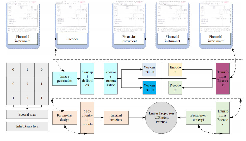
In era of big data, the computer vision-assisted textual extraction techniques for financial invoices have been a major concern. Currently, such tasks are mainly implemented via traditional image processing techniques. However, they highly rely on manual feature extraction and are mainly developed for specific financial invoice scenes. The general applicability and robustness are the major challenges faced by them. As consequence, deep learning can adaptively learn feature representation for different scenes and be utilized to deal with the above issue. As a consequence, this work introduces a classic pre-training model named visual transformer to construct a lightweight recognition model for this purpose. First, we use image processing technology to preprocess the bill image. Then, we use a sequence transduction model to extract information. The sequence transduction model uses a visual transformer structure. In the stage target location, the horizontal-vertical projection method is used to segment the individual characters, and the template matching is used to normalize the characters. In the stage of feature extraction, the transformer structure is adopted to capture relationship among fine-grained features through multi-head attention mechanism. On this basis, a text classification procedure is designed to output detection results. Finally, experiments on a real-world dataset are carried out to evaluate performance of the proposal and the obtained results well show the superiority of it. Experimental results show that this method has high accuracy and robustness in extracting financial bill information.

References

[1]	Y. Chen, C. Liu, W. Huang, S. Cheng, R. Arcucci, Z. Xiong, Generative text-guided 3d vision-language pretraining for unified medical image segmentation, preprint, arXiv: 2306.04811. https://doi.org/10.48550/arXiv.2306.04811
[2]	Z. Wan, C. Liu, M. Zhang, J. Fu, B. Wang, S. Cheng, et al., Med-unic: Unifying cross-lingual medical vision-language pre-training by diminishing bias, preprint, arXiv: 2305.19894. https://doi.org/10.48550/arXiv.2305.19894
[3]	C. Liu, S. Cheng, C. Chen, M. Qiao, W. Zhang, A. Shah, et al., M-FLAG: medical vision-language pre-training with frozen language models and latent space geometry optimization, preprint, arXiv: 2307.08347. https://doi.org/10.48550/arXiv.2307.08347
[4]	Z. Guo, K. Yu, N. Kumar, W. Wei, S. Mumtaz, M. Guizani, Deep distributed learning-based poi recommendation under mobile edge networks, IEEE Internet Things J., 10 (2023), 303–317. https://doi.org/10.1109/JIOT.2022.3202628 doi: 10.1109/JIOT.2022.3202628
[5]	Y. Jin, L. Hou, Y. Chen, A time series transformer based method for the rotating machinery fault diagnosis, Neurocomputing, 494 (2022), 379–395. https://doi.org/10.1016/j.neucom.2022.04.111 doi: 10.1016/j.neucom.2022.04.111
[6]	Q. Li, L. Liu, Z. Guo, P. Vijayakumar, F. Taghizadeh-Hesary, K. Yu, Smart assessment and forecasting framework for healthy development index in urban cities, Cities, 131 (2022), 103971. https://doi.org/10.1016/j.cities.2022.103971 doi: 10.1016/j.cities.2022.103971
[7]	J. Zhang, X. Liu, W. Liao, X. Li, Deep-learning generation of poi data with scene images, ISPRS J. Photogramm. Remote Sens., 188 (2022), 201–219. https://doi.org/10.1016/j.isprsjprs.2022.04.004 doi: 10.1016/j.isprsjprs.2022.04.004
[8]	Z. Guo, Y. Shen, S. Wan, W. Shang, K. Yu, Hybrid intelligence-driven medical image recognition for remote patient diagnosis in internet of medical things, IEEE J. Biomed. Health. Inf., 26 (2022), 5817–5828. https://doi.org/10.1109/JBHI.2021.3139541 doi: 10.1109/JBHI.2021.3139541
[9]	D. Zhang, X. Gao, A digital twin dosing system for iron reverse flotation, J. Manuf. Syst., 63 (2022), 238–249. https://doi.org/10.1016/j.jmsy.2022.03.006 doi: 10.1016/j.jmsy.2022.03.006
[10]	Z. Guo, Q. Zhang, F. Ding, X. Zhu, K. Yu, A novel fake news detection model for context of mixed languages through multiscale transformer, IEEE Trans. Comput. Social Syst., 2023. https://doi.org/10.1109/TCSS.2023.3298480 doi: 10.1109/TCSS.2023.3298480
[11]	X. Sun, Y. Zou, S. Wang, H. Su, B. Guan, A parallel network utilizing local features and global representations for segmentation of surgical instruments, Int. J. Comput. Assisted Radiol. Surg., 17 (2022), 1903–1913. https://doi.org/10.1007/s11548-022-02687-z doi: 10.1007/s11548-022-02687-z
[12]	Z. Chen, J. Chen, S. Liu, Y. Feng, S. He, E. Xu, Multi-channel calibrated transformer with shifted windows for few-shot fault diagnosis under sharp speed variation, ISA Trans., 131 (2022), 501–515. https://doi.org/10.1016/j.isatra.2022.04.043 doi: 10.1016/j.isatra.2022.04.043
[13]	M. Sun, L. Xu, R. Luo, Y. Lu, W. Jia, Ghformer-net: Towards more accurate small green apple/begonia fruit detection in the nighttime, J. King Saud Univ.-Comput. Inf. Sci., 34 (2022), 4421–4432. https://doi.org/10.1016/j.jksuci.2022.05.005 doi: 10.1016/j.jksuci.2022.05.005
[14]	D. Chen, J. Zheng, G. Wei, F. Pan, Extracting predictive representations from hundreds of millions of molecules, J. Phys. Chem. Lett., 12 (2021), 10793–10801.
[15]	N. P. Tigga, S. Garg, Efficacy of novel attention-based gated recurrent units transformer for depression detection using electroencephalogram signals, Health Inf. Sci. Syst., 11 (2023). https://doi.org/10.1007/s13755-022-00205-8 doi: 10.1007/s13755-022-00205-8
[16]	B. Wang, Q. Li, Z. You, Self-supervised learning based transformer and convolution hybrid network for one-shot organ segmentation, Neurocomputing, 527 (2023). https://doi.org/10.1016/j.neucom.2022.12.028 doi: 10.1016/j.neucom.2022.12.028
[17]	S. Xiao, S. Wang, Z. Huang, Y. Wang, H. Jiang, Two-stream transformer network for sensor-based human activity recognition, Neurocomputing, 512 (2022), 253–268. https://doi.org/10.1016/j.neucom.2022.09.099 doi: 10.1016/j.neucom.2022.09.099
[18]	M. Mao, R. Zhang, H. Zheng, T. Ma, Y. Peng, E. Ding, et al., Dual-stream network for visual recognition, Adv. Neural Inf. Process. Syst., 34 (2021), 25346–25358.
[19]	R. Kozik, M. Pawlicki, M. Chorś, A new method of hybrid time window embedding with transformer-based traffic data classification in iot-networked environment, Pattern Anal. Appl., 24 (2021), 1441–1449. https://doi.org/10.1007/s10044-021-00980-2 doi: 10.1007/s10044-021-00980-2
[20]	A. A. Khan, R. Jahangir, R. Alroobaea, S. Y. Alyahyan, A. H. Almulhi, M. Alsafyani, et al., An efficient text-independent speaker identification using feature fusion and transformer model, Comput. Mater. Contin., 75 (2023), 4085–4100.
[21]	D. Li, B. Li, S. Long, H. Feng, T. Xi, S. Kang, et al., Rice seedling row detection based on morphological anchor points of rice stems, Biosyst. Eng., 226 (2023), 71–85. https://doi.org/10.1016/j.biosystemseng.2022.12.012 doi: 10.1016/j.biosystemseng.2022.12.012
[22]	Y. Yang, J. Yu, H. Jiang, W. Han, J. Zhang, W. Jiang, A contrastive triplet network for automatic chest x-ray reporting, Neurocomputing, 502 (2022), 71–83. https://doi.org/10.1016/j.neucom.2022.06.063 doi: 10.1016/j.neucom.2022.06.063
[23]	B. Zhang, J. Abbing, A. Ghanem, D. Fer, J. Barker, R. Abukhalil, et al., Towards accurate surgical workflow recognition with convolutional networks and transformers, Comput. Methods Biomech. Biomed. Eng.: Imaging Visualization, 10 (2022), 349–356. https://doi.org/10.1080/21681163.2021.2002191 doi: 10.1080/21681163.2021.2002191
[24]	X. Pan, X. Gao, H. Wang, W. Zhang, Y. Mu, X. He, Temporal-based swin transformer network for workflow recognition of surgical video, Int. J. Comput. Assisted Radiol. Surg., 18 (2023), 139–147.
[25]	Y. J. Shin, S. B. Jeong, H. I. Seo, W. Y. Kim, D. H. Seo, A study on handwritten parcel delivery invoice understanding model, J. Adv. Mar. Eng. Technol. (JAMET), 46 (2022), 430–438. https://doi.org/10.5916/jamet.2022.46.6.430 doi: 10.5916/jamet.2022.46.6.430
[26]	Y. Liu, T. Bai, Y. Tian, Y. Wang, J. Wang, X. Wang, et al., Segdq: Segmentation assisted multi-object tracking with dynamic query-based transformers, Neurocomputing, 481 (2022), 91–101. https://doi.org/10.1016/j.neucom.2022.01.073 doi: 10.1016/j.neucom.2022.01.073
[27]	L. Tang, X. Xiang, H. Zhang, M. Gong, J. Ma, Divfusion: Darkness-free infrared and visible image fusion, Inf. Fusion, 91 (2023), 477–493. https://doi.org/10.1016/j.inffus.2022.10.034 doi: 10.1016/j.inffus.2022.10.034
[28]	H. Jiang, M. Gao, H. Li, R. Jin, H. Miao, J. Liu, Multi-learner based deep meta-learning for few-shot medical image classification, IEEE J. Biomed. Health Inf., 27 (2023), 17–28. https://doi.org/10.1109/JBHI.2022.3215147 doi: 10.1109/JBHI.2022.3215147
[29]	M. Luo, H. Wu, H. Huang, W. He, R. He, Memory-modulated transformer network for heterogeneous face recognition, IEEE Trans. Inf. Forensics Secur., 17 (2022), 2095–2109. https://doi.org/10.1109/TIFS.2022.3177960 doi: 10.1109/TIFS.2022.3177960
[30]	J. Izquierdo-Domenech, J. Linares-Pellicer, J. Orta-Lopez, Towards achieving a high degree of situational awareness and multimodal interaction with ar and semantic ai in industrial applications, Multimedia Tools Appl., 82 (2023), 15875–15901. https://doi.org/10.1007/s11042-022-13803-1 doi: 10.1007/s11042-022-13803-1
[31]	Z. Yu, Y. Shen, J. Shi, H. Zhao, Y. Cui, J. Zhang, et al., Physformer++: Facial video-based physiological measurement with slowfast temporal difference transformer, Int. J. Comput. Vision, 131 (2023), 1307–1330.
[32]	H. Ji, X. Cui, W. Ren, L. Liu, W. Wang, Visual inspection for transformer insulation defects by a patrol robot fish based on deep learning, IET Sci. Meas. Technol., 15 (2021), 606–618. https://doi.org/10.1049/smt2.12062 doi: 10.1049/smt2.12062
[33]	Y. Wu, K. Liao, J. Chen, J. Wang, D. Z. Chen, H. Gao, et al., D-former: A u-shaped dilated transformer for 3d medical image segmentation, Neural Comput. Appl., 35 (2023), 1931–1944. https://doi.org/10.1007/s00521-022-07859-1 doi: 10.1007/s00521-022-07859-1
[34]	C. Liu, Z. Mao, A. Liu, T. Zhang, B. Wang, Y. Zhang, Focus your attention: A bidirectional focal attention network for image-text matching, in Proceedings of the 27th ACM International Conference on Multimedia, ACM, (2019), 3–11. https://doi.org/10.1145/3343031.3350869
[35]	C. Liu, Z. Mao, T. Zhang, H. Xie, B. Wang, Y. Zhang, Graph structured network for image-text matching, in Proceedings of the IEEE/CVF Conference on Computer Vision and Pattern Recognition, (2020), 10918–10927. https://doi.org/10.1109/CVPR42600.2020.01093
[36]	H. Diao, Y. Zhang, L. Ma, H. Lu, Similarity reasoning and filtration for image-text matching, in Proceedings of the AAAI Conference on Artificial Intelligence, 35 (2021), 1218–1226. https://doi.org/10.1609/aaai.v35i2.16209

Reader Comments

Your name:*

Email:*
© 2023 the Author(s), licensee AIMS Press. This is an open access article distributed under the terms of the Creative Commons Attribution License (http://creativecommons.org/licenses/by/4.0)