Dynamics of an SEIR model with media coverage mediated nonlinear infectious force

Jingli Xie; Hongli Guo; Meiyang Zhang; Jingli Xie; Hongli Guo; Meiyang Zhang

doi:10.3934/mbe.2023654

Mathematical Biosciences and Engineering

2023, Volume 20, Issue 8: 14616-14633. doi: 10.3934/mbe.2023654

Previous Article Next Article

Research article Special Issues

Dynamics of an SEIR model with media coverage mediated nonlinear infectious force

College of Mathematics and Statistics, Jishou University, Jishou, Hunan 416000, China

Academic Editor: Xiang-Sheng Wang

Received: 10 April 2023 Revised: 04 June 2023 Accepted: 21 June 2023 Published: 05 July 2023

Media coverage can greatly impact the spread of infectious diseases. Taking into consideration the impacts of media coverage, we propose an SEIR model with a media coverage mediated nonlinear infection force. For this novel disease model, we identify the basic reproduction number using the next generation matrix method and establish the global threshold results: If the basic reproduction number $ \mathcal{R}_{0} < 1 $, then the disease-free equilibrium $ P_{0} $ is stable, and the disease dies out. If $ \mathcal{R}_{0} > 1 $, then the endemic equilibrium $ P^{*} $ is stable, and the disease persists. Sensitivity analysis indicates that the basic reproduction number $ \mathcal{R}_{0} $ is most sensitive to the population recruitment rate $ \Lambda $ and the disease transmission rate $ \beta _{1} $.
- media influence,
- SEIR model,
- incubation period,
- sensitivity analysis,
- stability
Citation: Jingli Xie, Hongli Guo, Meiyang Zhang. Dynamics of an SEIR model with media coverage mediated nonlinear infectious force[J]. Mathematical Biosciences and Engineering, 2023, 20(8): 14616-14633. doi: 10.3934/mbe.2023654

Related Papers:

Abstract

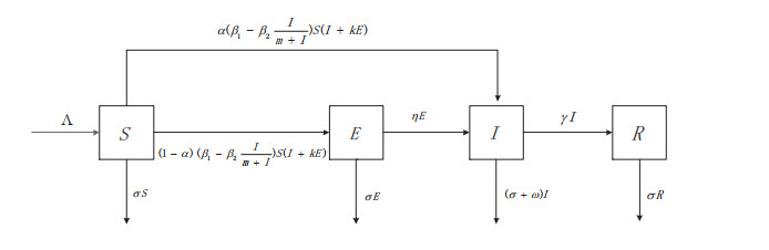
Media coverage can greatly impact the spread of infectious diseases. Taking into consideration the impacts of media coverage, we propose an SEIR model with a media coverage mediated nonlinear infection force. For this novel disease model, we identify the basic reproduction number using the next generation matrix method and establish the global threshold results: If the basic reproduction number $ \mathcal{R}_{0} < 1 $, then the disease-free equilibrium $ P_{0} $ is stable, and the disease dies out. If $ \mathcal{R}_{0} > 1 $, then the endemic equilibrium $ P^{*} $ is stable, and the disease persists. Sensitivity analysis indicates that the basic reproduction number $ \mathcal{R}_{0} $ is most sensitive to the population recruitment rate $ \Lambda $ and the disease transmission rate $ \beta _{1} $.

References

[1]	J. M. Tchuenche, N. Dube, C. P. Bhunu, R. J. Smith, C. T. Bauch, The impact of media coverage on the transmission dynamics of human influenza, BMC Public Health, 11 (2011), 1–14. https://doi.org/10.1186/1471-2458-11-S1-S5 doi: 10.1186/1471-2458-11-S1-S5
[2]	W. K. Zhou, Y. N. Xiao, J. M. Heffernan, Optimal media reporting intensity on mitigating spread of an emerging infectious disease, PLoS One, 14 (2019), e0213898. https://doi.org/10.1371/journal.pone.0213898 doi: 10.1371/journal.pone.0213898
[3]	R. S. Liu, J. H. Wu, H. P. Zhu, Media/psychological impact on multiple outbreaks of emerging infectious diseases, Comput. Math. Methods Med., 8 (2007), 153–164. https://doi.org/10.1080/17486700701425870 doi: 10.1080/17486700701425870
[4]	D. M. Xiao, S. G. Ruan, Global analysis of an epidemic model with nonmonotone incidence rate, Math. Biosci., 208 (2007), 419–429. https://doi.org/10.1016/j.mbs.2006.09.025 doi: 10.1016/j.mbs.2006.09.025
[5]	J. A. Cui, X. Tao, H. P. Zhu, An SIS infection model incorporating media coverage, Rocky Mt. J. Math., 38 (2008), 1323–1334. https://doi.org/10.1216/RMJ-2008-38-5-1323 doi: 10.1216/RMJ-2008-38-5-1323
[6]	J. Cui, Z. Wu, An SIRS model for assessing impact of media coverage, Abstr. Appl. Anal., 2014 (2014). https://doi.org/10.1155/2014/424610
[7]	Y. Wang, J. Cao, Z. Jin, H. Zhang, G. Q. Sun, Impact of media coverage on epidemic spreading in complex networks, Physica A, 392 (2013), 5824–5835. https://doi.org/10.1016/j.physa.2013.07.067 doi: 10.1016/j.physa.2013.07.067
[8]	S. R. Gani, S. V. Halawar, Optimal control for the spread of infectious disease: the role of awareness programs by media and antiviral treatment, Optim. Control Appl. Methods, 39 (2018), 1407–1430. https://doi.org/10.1002/oca.2418 doi: 10.1002/oca.2418
[9]	A. Kumar, P. K. Srivastava, Y. P. Dong, Y. Takeuchi, Optimal control of infectious disease: information-induced vaccination and limited treatment, Physica A, 542 (2020), 123196. https://doi.org/10.1016/j.physa.2019.123196 doi: 10.1016/j.physa.2019.123196
[10]	S. S. Shanta, M. H. A. Biswas, The impact of media awareness in controlling the spread of infectious diseases in terms of SIR model, Math. Modell. Eng. Probl., 7 (2020), 368–376. https://doi.org/10.18280/mmep.070306 doi: 10.18280/mmep.070306
[11]	W. Wang, X. Q. Zhao, Threshold dynamics for compartmental epidemic models in periodic environments, J. Dyn. Differ. Equations, 20 (2008), 699–717. https://doi.org/10.1007/s10884-008-9111-8 doi: 10.1007/s10884-008-9111-8
[12]	W. Xing, J. F. Gao, Q. S. Yan, Q. H. Zhou, Z. H. Yang, An epidemic model with saturated media/psychological impact (in Chinese), J. Northwest Univ. (Nat. Sci. Ed.), 48 (2018), 639–643. Available from: https://kns.cnki.net/kcms/detail/61.1072.N.20181015.1716.006.html.
[13]	Q. L. Yan, S. Y. Tang, S. Gabriele, J. H. Wu, Media coverage and hospital notifications: correlation analysis and optimal media impact duration to manage a pandemic, J. Theor. Biol., 390 (2016), 1–13. https://doi.org/10.1016/j.jtbi.2015.11.002 doi: 10.1016/j.jtbi.2015.11.002
[14]	Q. L. Yan, Y. L. Tang, D. D. Yan, J. Y. Wang, L. Q. Yang, X. P. Yang, et al., Impact of media reports on the early spread of COVID-19 epidemic, J. Theor. Biol., 502 (2020). https://doi.org/10.1016/j.jtbi.2020.110385
[15]	I. Ghosh, P. K. Tiwari, S. Samanta, I. M. Elmojtaba, N. Al-Salti, J. Chattopadhyay, A simple SI-type model for HIV/AIDS with media and self-imposed psychological fear, J. Math. Biosci., 306 (2018), 160–169. https://doi.org/10.1016/j.mbs.2018.09.014 doi: 10.1016/j.mbs.2018.09.014
[16]	S. Latifah, D. Aldila, W. Giyarti, H. Tasman, Mathematical study for an infectious disease with awareness-based SIS-M model, J. Phys. Conf. Ser., 1747 (2021), 012017. https://doi.org/10.1088/1742-6596/1747/1/012017 doi: 10.1088/1742-6596/1747/1/012017
[17]	G. O. Agaba, Y. N. Kyrychko, K. B. Blyuss, Mathematical model for the impact of awareness on the dynamics of infectious diseases, Math. Biosci., 286 (2017), 22–30. https://doi.org/10.1016/j.mbs.2017.01.009 doi: 10.1016/j.mbs.2017.01.009
[18]	P. van den Driessche, J. Watmough, Reproduction numbers and sub-threshold endemic equilibria for compartmental models of disease transmission, Math. Biosci., 180 (2002), 29–48. https://doi.org/10.1016/S0025-5564(02)00108-6 doi: 10.1016/S0025-5564(02)00108-6
[19]	C. Castillo-Chaves, H. R. Thieme, Asymptotically autonomous epidemic models, in Mathematical Population Dynamics: Analysis of Heterogeneity. Volume One, Theory of Epidemics, (1995), 33–50. Available from: https://www.researchgate.net/publication/221711274.
[20]	M. Y. Li, H. Smith, L. C. Wang, Global dynamics of an SEIR epidemic model with vertical transmission, SIAM J. Appl. Math., 62 (2001), 58–69. https://doi.org/10.1137/S0036139999359860 doi: 10.1137/S0036139999359860
[21]	N. Chitnis, J. M. Hyman, J. M. Cushing, Determining important parameters in the spread of malaria through the sensitivity analysis of a mathematical model, Bull. Math. Biol., 70 (2008), 1272–1296. https://doi.org/10.1007/s11538-008-9299-0 doi: 10.1007/s11538-008-9299-0
[22]	Y. N. Sun, Analysis of Several Models on the Infectious Diseases with the Effect of Awareness (in Chinese), Master's thesis, North University of China, 2021. https://doi.org/10.27470/d.cnki.ghbgc.2021.001026
[23]	B. Tang, F. Xia, S. Y. Tang, N. L. Bragazzi, Q. Li, X. D. Sun, et al., The effectiveness of quarantine and isolation determine the trend of the COVID-19 epidemics in the final phase of the current outbreak in China, Int. J. Infect. Dis., 95 (2020), 288–293. https://doi.org/10.1016/j.ijid.2020.03.018 doi: 10.1016/j.ijid.2020.03.018
[24]	M. Mandal, S. Jana, S. K. Nandi, A. Khatua, S. Adak, T. K. Kar, A model based study on the dynamics of COVID-19: prediction and control, Chaos, Solitons Fractals, 136 (2020), 109889. https://doi.org/10.1016/j.chaos.2020.109889 doi: 10.1016/j.chaos.2020.109889
[25]	B. Tang, X. Wang, Q. Li, N. L. Bragazzi, S. Y. Tang, Y. N. Xiao, et al., Estimation of the transmission risk of the 2019-nCoV and its implication for public health interventions, J. Clin. Med., 9 (2020), 462. https://doi.org/10.3390/jcm9020462 doi: 10.3390/jcm9020462

Reader Comments

Your name:*

Email:*
© 2023 the Author(s), licensee AIMS Press. This is an open access article distributed under the terms of the Creative Commons Attribution License (http://creativecommons.org/licenses/by/4.0)