High quality medical images play an important role in intelligent medical analyses. However, the difficulty of acquiring medical images with professional annotation makes the required medical image datasets, very expensive and time-consuming. In this paper, we propose a semi-supervised method, $ {\mathrm{C}\mathrm{A}\mathrm{U}}^{+} $, which is a consensus model of augmented unlabeled data for cardiac image segmentation. First, the whole is divided into two parts: the segmentation network and the discriminator network. The segmentation network is based on the teacher student model. A labeled image is sent to the student model, while an unlabeled image is processed by CTAugment. The strongly augmented samples are sent to the student model and the weakly augmented samples are sent to the teacher model. Second, $ {\mathrm{C}\mathrm{A}\mathrm{U}}^{+} $ adopts a hybrid loss function, which mixes the supervised loss for labeled data with the unsupervised loss for unlabeled data. Third, an adversarial learning is introduced to facilitate the semi-supervised learning of unlabeled images by using the confidence map generated by the discriminator as a supervised signal. After evaluating on an automated cardiac diagnosis challenge (ACDC), our proposed method $ {\mathrm{C}\mathrm{A}\mathrm{U}}^{+} $ has good effectiveness and generality and $ {\mathrm{C}\mathrm{A}\mathrm{U}}^{+} $ is confirmed to have a improves dice coefficient (DSC) by up to 18.01, Jaccard coefficient (JC) by up to 16.72, relative absolute volume difference (RAVD) by up to 0.8, average surface distance (ASD) and 95% Hausdorff distance ($ {HD}_{95} $) reduced by over 50% than the latest semi-supervised learning methods.
Citation: Wenli Cheng, Jiajia Jiao. An adversarially consensus model of augmented unlabeled data for cardiac image segmentation (CAU+)[J]. Mathematical Biosciences and Engineering, 2023, 20(8): 13521-13541. doi: 10.3934/mbe.2023603
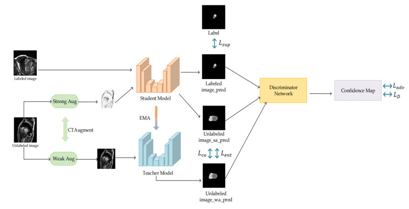
High quality medical images play an important role in intelligent medical analyses. However, the difficulty of acquiring medical images with professional annotation makes the required medical image datasets, very expensive and time-consuming. In this paper, we propose a semi-supervised method, $ {\mathrm{C}\mathrm{A}\mathrm{U}}^{+} $, which is a consensus model of augmented unlabeled data for cardiac image segmentation. First, the whole is divided into two parts: the segmentation network and the discriminator network. The segmentation network is based on the teacher student model. A labeled image is sent to the student model, while an unlabeled image is processed by CTAugment. The strongly augmented samples are sent to the student model and the weakly augmented samples are sent to the teacher model. Second, $ {\mathrm{C}\mathrm{A}\mathrm{U}}^{+} $ adopts a hybrid loss function, which mixes the supervised loss for labeled data with the unsupervised loss for unlabeled data. Third, an adversarial learning is introduced to facilitate the semi-supervised learning of unlabeled images by using the confidence map generated by the discriminator as a supervised signal. After evaluating on an automated cardiac diagnosis challenge (ACDC), our proposed method $ {\mathrm{C}\mathrm{A}\mathrm{U}}^{+} $ has good effectiveness and generality and $ {\mathrm{C}\mathrm{A}\mathrm{U}}^{+} $ is confirmed to have a improves dice coefficient (DSC) by up to 18.01, Jaccard coefficient (JC) by up to 16.72, relative absolute volume difference (RAVD) by up to 0.8, average surface distance (ASD) and 95% Hausdorff distance ($ {HD}_{95} $) reduced by over 50% than the latest semi-supervised learning methods.

| [1] |
C. Chen, C. Qin, H. Qiu, G. Tarroni, J. Duan, W. Bai, et al., Deep learning for cardiac image segmentation: A review, Front. Cardiovasc. Med., 7 (2020), 25. https://doi.org/10.3389/fcvm.2020.00025 doi: 10.3389/fcvm.2020.00025

|
| [2] |
C. A. Miller, P. Jordan, A. Borg, R. Argyle, D. Clark, K. Pearce, et al., Quantification of left ventricular indices from SSFP cine imaging: Impact of real-world variability in analysis methodology and utility of geometric modeling, J. Magn. Reson. Imag., 37 (2013), 1213–1222. https://doi.org/10.1002/jmri.23892 doi: 10.1002/jmri.23892
|
| [3] |
S. Queirós, D. Barbosa, B. Heyde, P. Morais, J. L. Vilaça, D. Friboulet, et al., Fast automatic myocardial segmentation in 4D cine CMR datasets, Med. Image Anal., 18 (2014), 1115–1131. https://doi.org/10.1016/j.media.2014.06.001 doi: 10.1016/j.media.2014.06.001
|
| [4] | D. H. N. Nham, M. N. Trinh, T. T. Tran, V. T. Pham, T. T. Tran, A modified FCN-based method for Left Ventricle endocardium and epicardium segmentation with new block modules, in 2021 8th NAFOSTED Conference on Information and Computer Science (NICS), (2021), 392–397. https://doi.org/10.1109/NICS54270.2021.9701571 |
| [5] |
Z. F. Shaaf, M. M. A. Jamil, R. Ambar, A. A. Alattab, A. A. Yahya, Y. Asiri, Automatic left ventricle segmentation from short-axis cardiac MRI images based on fully convolutional neural network, Diagnostics, 12 (2022), 414. https://doi.org/10.3390/diagnostics12020414 doi: 10.3390/diagnostics12020414
|
| [6] |
P. Daudé, P. Ancel, S. C. Gouny, A. Jacquier, F. Kober, A. Dutour, et al., Deep-learning segmentation of epicardial adipose tissue using four-chamber cardiac magnetic resonance imaging, Diagnostics, 12 (2022), 126. https://doi.org/10.3390/diagnostics12010126 doi: 10.3390/diagnostics12010126
|
| [7] |
Z. F. Shaaf, M. M. A. Jamil, R. Ambar, A. A. Alattab, A. A. Yahya, Y. Asiri, Automatic left ventricle segmentation from short-axis cardiac MRI images based on fully convolutional neural network, Diagnostics, 12 (2022), 414. https://doi.org/10.3390/diagnostics12020414 doi: 10.3390/diagnostics12020414
|
| [8] |
Z. Fu, J. Zhang, R. Luo, Y. Sun, D. Deng, L. Xia. TF-Unet: An automatic cardiac MRI image segmentation method, Math. Biosci. Eng., 19 (2022), 5207–5222. https://doi.org/10.3934/mbe.2022244 doi: 10.3934/mbe.2022244
|
| [9] |
D. Abdelrauof, M. Essam, M. Elattar, Light-weight localization and scale-independent multi-gate UNET segmentation of left and right ventricles in MRI images, Cardiovasc. Eng. Tech., 13 (2022), 393–406. https://doi.org/10.1007/s13239-021-00591-2 doi: 10.1007/s13239-021-00591-2
|
| [10] |
Z. Liu, X. He, Y. Lu, Combining UNet 3+ and transformer for left ventricle segmentation via signed distance and focal loss, Appl. Sci., 12 (2022), 9208. https://doi.org/10.3390/app12189208 doi: 10.3390/app12189208
|
| [11] | W. Cheng, J. Jiao, CAU: A consensus model of augmented unlabeled data for medical image segmentation, in 2022 7th International Conference on Image, Vision and Computing (ICIVC), (2022), 368–374. https://doi.org/10.1109/ICIVC55077.2022.9886218 |
| [12] | W. Hung, Y. Tsai, Y. Liou, Y. Lin, M. Yang, Adversarial learning for semi-supervised semantic segmentation, preprint, arXiv: 1802.07934. https://doi.org/10.48550/arXiv.1802.07934 |
| [13] | D. H. Lee, Pseudo-label: The simple and efficient semi-supervised learning method for deep neural networks, in ICML 2013 Workshop: Challenges in Representation Learning (WREPL), 2013. |
| [14] | A. Tarvainen. H. Valpola, Mean teachers are better role models: Weightaveraged consistency targets improve semi-supervised deep learning results, Adv. Neural Inf. Process. Syst., 30 (2017). |
| [15] | D. Berthelot, N. Carlini, I. Goodfellow, N. Papernot, A. Oliver, C. Raffel, MixMatch: A holistic approach to semi-supervised learning, Adv. Neural Inf. Process. Syst., 32 (2019). |
| [16] | D. Berthelot, N. Carlini, E. D. Cubuk, A. Kurakin, K. Sohn, H. Zhang, et al., ReMixMatch: Semi-supervised learning with distribution alignment and augmentation anchoring, preprint, arXiv: 1911.09785. https://doi.org/10.48550/arXiv.1911.09785 |
| [17] | K. Sohn, D. Berthelot, C. Li, Z. Zhang, N. Carlini, E. D. Cubuk, et al., FixMatch: Simplifying semi-supervised learning with consistency and confidence, Adv. Neural Inf. Process. Syst., 33 (2020), 596–608. |
| [18] | E. D. Cubuk, B. Zoph, D. Mane, V. Vasudevan, Q. V. Le, AutoAugment: Learning augmentation policies from data, preprint, arXiv: 1805.09501. https://doi.org/10.48550/arXiv.1805.09501 |
| [19] | E. D. Cubuk, B. Zoph, J. Shlens, Q. V. Le, Randaugment: Practical automated data augmentation with a reduced search space, in Proceedings of the IEEE/CVF conference on computer vision and pattern recognition workshops, (2020), 702–703. https://doi.org/10.1109/CVPRW50498.2020.00359 |
| [20] |
G. Chen, J. Ru, Y. Zhou, I. Rekik, Z. Pan, X. Liu, et al., Mtans: Multi-scale mean teacher combined adversarial network with shape-aware embedding for semi-supervised brain lesion segmentation, NeuroImage, 244 (2021), 118568. https://doi.org/10.1016/j.neuroimage.2021.118568 doi: 10.1016/j.neuroimage.2021.118568
|
| [21] | Y. Zhang, L. Yang, J. Chen, M. Fredericksen, D. P. Hughes, D. Z. Chen, Deep adversarial networks for biomedical image segmentation utilizing unannotated images, in International Conference on Medical Image Computing and Computer-Assisted Intervention, Springer, (2017), 408–416. https://doi.org/10.1007/978-3-319-66179-7_47 |
| [22] |
D. Zhai, B. Hu, X. Gong, H. Zou, J. Luo, ASS-GAN: Asymmetric semi-supervised GAN for breast ultrasound image segmentation, Neurocomputing, 493 (2022), 204–216. https://doi.org/10.1016/j.neucom.2022.04.021 doi: 10.1016/j.neucom.2022.04.021
|
| [23] |
K. Shen, H. Quan, J. Han, M. Wu, URO-GAN: An untrustworthy region optimization approach for adipose tissue segmentation based on adversarial learning, Appl. Intell., 52 (2022), 10247–10269. https://doi.org/10.1007/s10489-021-02976-1 doi: 10.1007/s10489-021-02976-1
|
| [24] |
C. Xu, Y. Wang, D. Zhang, L. Han, Y. Zhang, J. Chen, et al., BMAnet: Boundary mining with adversarial learning for semi-supervised 2D myocardial infarction segmentation, IEEE J. Biomed. Health Inf., 27 (2023), 87–96. https://doi.org/10.1109/JBHI.2022.3215536 doi: 10.1109/JBHI.2022.3215536
|
| [25] | O. Ronneberger, P. Fischer, T. Brox, U-net: Convolutional networks for biomedical image segmentation, in Medical Image Computing and Computer-Assisted Intervention—MICCAI 2015, (2015), 234–241. https://doi.org/10.1007/978-3-319-24574-4_28 |
| [26] | X. Luo, J. Chen, T. Song, G.Wang, Semi-supervised medical image segmentation through dual-task consistency, in Proceedings of the AAAI Conference on Artificial Intelligence, 35 (2021), 8801–8809. https://doi.org/10.1609/aaai.v35i10.17066 |
| [27] |
C. E. Shannon, A mathematical theory of communication, SIGMOBILE Mob. Comput. Commun. Rev., 5 (2001), 3–55. https://doi.org/10.1145/584091.584093 doi: 10.1145/584091.584093
|
| [28] | Y. Grandvalet, Y. Bengio, Semi-supervised learning by entropy minimization, Adv. Neural Inf. Process. Syst., 2004 (2004), 17. |
| [29] | W. Bai, O. Oktay, M. Sinclair, H. Suzuki, M. Rajchl, G. Tarroni, et al., Semi-supervised learning for network-based cardiac mr image segmentation, in Medical Image Computing and Computer-Assisted Intervention—MICCAI 2017, (2017), 253–260. https://doi.org/10.1007/978-3-319-66185-8_29 |
| [30] | R. K. Meleppat, M. V. Matham, L. K. Seah, Optical frequency domain imaging with a rapidly swept laser in the 1300nm bio-imaging window, in International Conference on Optical and Photonic Engineering (icOPEN 2015), (2015), 721–729. https://doi.org/10.1117/12.2190530 |
| [31] |
K. M. Ratheesh, L. K. Seah, V. M. Murukeshan, Spectral phase-based automatic calibration scheme for swept source-based optical coherence tomography systems, Phys. Med. Biol., 61 (2016), 7652. https://doi.org/10.1088/0031-9155/61/21/7652 doi: 10.1088/0031-9155/61/21/7652
|
| [32] |
R. K. Meleppat, M. V. Matham, L. K. Seah, An efficient phase analysis-based wavenumber linearization scheme for swept source optical coherence tomography systems, Laser Phys. Lett., 12 (2015), 055601. https://doi.org/10.1088/1612-2011/12/5/055601 doi: 10.1088/1612-2011/12/5/055601
|
| [33] | R. K. Meleppat, P. Prabhathan, S. L. Keey, M. V. Matham, Plasmon resonant silica-coated silver nanoplates as contrast agents for optical coherence tomography, 12 (2016), 1929–1937. https://doi.org/10.1166/jbn.2016.2297 |


Figures(5) / Tables(6)

Wenli Cheng, Jiajia Jiao. An adversarially consensus model of augmented unlabeled data for cardiac image segmentation (CAU+)[J]. Mathematical Biosciences and Engineering, 2023, 20(8): 13521-13541. doi: 10.3934/mbe.2023603


 DownLoad: