The Internet of Things (IoT) refers to the use of various communication technologies to achieve the interconnection of everything in cyberspace, and to achieve smart home and intelligent transportation, thus generating unprecedented amounts of data. In the financial sharing center, all businesses can extract effective data from these massive databases for analysis, and use data analysis tools to collect business, financial, human, process, knowledge and social data. At present, various types of IT (Internet Technology) systems have been widely used in financial sharing centers. However, a large number of sensitive data have also been generated. In order to protect these sensitive data, there is a high requirement for the personal information of IT system operation and financial sharing center personnel. In order to protect user data privacy, the optimal and most effective use of IT systems is an important issue that must be considered in privacy management. At present, there are many algorithms to protect data and privacy, but the effect is not ideal. Considering the balance between privacy issues, this paper proposed a K-means clustering algorithm based on IoT public cloud privacy protection technology to analyze the performance management of financial sharing center. The research results showed that before the improvement, the average number of employees who were dissatisfied with the post training ability and information platform construction ability of the financial sharing center was 57.9 and 57.8% respectively, more than half of them. After the improvement of IoT based public cloud privacy protection, the average number of employees dissatisfied with the post training ability and information platform construction ability of the financial sharing center was 5 and 3.9%, far less than the data prior to the improvement. It showed that IoT public cloud privacy protection was conducive to the performance management of the financial sharing center, and the relationship between the two was positive.
Citation: Zhen Yu, Sheng-Huang Lin, Chia-Ching Cho, Changping Chen. Performance management algorithm of financial shared service center based on Internet of Things public cloud privacy protection[J]. Mathematical Biosciences and Engineering, 2023, 20(7): 12510-12528. doi: 10.3934/mbe.2023557
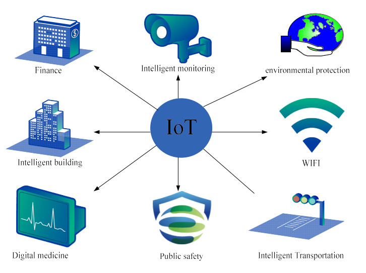
The Internet of Things (IoT) refers to the use of various communication technologies to achieve the interconnection of everything in cyberspace, and to achieve smart home and intelligent transportation, thus generating unprecedented amounts of data. In the financial sharing center, all businesses can extract effective data from these massive databases for analysis, and use data analysis tools to collect business, financial, human, process, knowledge and social data. At present, various types of IT (Internet Technology) systems have been widely used in financial sharing centers. However, a large number of sensitive data have also been generated. In order to protect these sensitive data, there is a high requirement for the personal information of IT system operation and financial sharing center personnel. In order to protect user data privacy, the optimal and most effective use of IT systems is an important issue that must be considered in privacy management. At present, there are many algorithms to protect data and privacy, but the effect is not ideal. Considering the balance between privacy issues, this paper proposed a K-means clustering algorithm based on IoT public cloud privacy protection technology to analyze the performance management of financial sharing center. The research results showed that before the improvement, the average number of employees who were dissatisfied with the post training ability and information platform construction ability of the financial sharing center was 57.9 and 57.8% respectively, more than half of them. After the improvement of IoT based public cloud privacy protection, the average number of employees dissatisfied with the post training ability and information platform construction ability of the financial sharing center was 5 and 3.9%, far less than the data prior to the improvement. It showed that IoT public cloud privacy protection was conducive to the performance management of the financial sharing center, and the relationship between the two was positive.

| [1] |
J. Sai, Research on big data audit based on financial sharing service model using fuzzy AHP, J. Intell. Fuzzy Syst., 40 (2021), 8237–8246. https://doi.org/10.3233/JIFS-189646 doi: 10.3233/JIFS-189646

|
| [2] |
G. Xie, Performance evaluation of cross-departmental data sharing in coastal cities based on big data era, J. Coastal Res., 107 (2020), 215–217. https://doi.org/10.2112/JCR-SI107-054.1 doi: 10.2112/JCR-SI107-054.1
|
| [3] |
L. Li, F. Yan, L. Li, Big data audit based on financial sharing service model, J. Intell. Fuzzy Syst., 39 (2020), 8997–9005. https://doi.org/10.3233/JIFS-189298 doi: 10.3233/JIFS-189298
|
| [4] |
Y. Huang, Analysis of the construction of management accounting system under the mode of financial sharing, Int. J. Edu. Humanit., 5 (2022), 205–207. https://doi.org/10.54097/ijeh.v5i2.2141 doi: 10.54097/ijeh.v5i2.2141
|
| [5] |
Y. Lu, Financial accounting intelligence management of internet of things enterprises based on data mining algorithm, J. Intell. Fuzzy Syst., 37 (2019), 5915–5923. https://doi.org/10.3233/JIFS-179173 doi: 10.3233/JIFS-179173
|
| [6] | Y. Cao, M. Sepideh, R. Shervin, G. Aria, Economic application of structural health monitoring and internet of things in efficiency of building information modeling, Smart Struct. Syst., 26 (2020), 559–573. |
| [7] | R. Ma, K. Misagh, G. Aria, Z. Yousef, B. Shahrizan, S. Abdellatif, et al., Assessment of composite beam performance using GWO–ELM metaheuristic algorithm, Eng. Comput., 2021 (2021), 1–17. |
| [8] | M. Armin, G. Aria, A. Soheila, Y. Maziar, B. Shahrizan, A. Hamid, Simulation of steel–concrete composite floor system behavior at elevated temperatures via multi-hybrid metaheuristic framework, Eng. Comput., 2021 (2021), 1–16. |
| [9] |
K. Tajziehchi, A. Ghabussi, H. Alizadeh, Control and optimization against earthquake by using genetic algorithm, J. Appl. Eng. Sci., 8 (2018), 73–78. https://doi.org/10.2478/jaes-2018-0010 doi: 10.2478/jaes-2018-0010
|
| [10] |
T. Zheng, X. A. Wang, W. Du, Z. Wang, M. Lv, An improved multi-copy cloud data auditing scheme and its application, J. King Saud Univ. Comput. Inf. Sci., 35 (2023), 120–130. https://doi.org/10.1016/j.jksuci.2023.01.021 doi: 10.1016/j.jksuci.2023.01.021
|
| [11] |
X. He, M. Guo, N. Nedjah, J. Zhang, P. Li, Vehicle and pedestrian detection algorithm based on lightweight YOLOv3-promote and semi-precision acceleration, IEEE Trans. Intell. Trans. Syst., 23 (2022), 19760–19771. https://doi.org/10.1109/TITS.2021.3137253 doi: 10.1109/TITS.2021.3137253
|
| [12] | Q. Chen, Study on the practice of corporate finance sharing center-vanke company as an example, Front. Econ. Manage., 2 (2021), 93–100. |
| [13] |
V. Mohagheghi, S. M. Mousavi, R. Shahabi-Shahmiri, Sustainable project portfolio selection and optimization with considerations of outsourcing decisions, financing options and staff assignment under interval type-2 fuzzy uncertainty, Neural Comput. Appl., 34 (2022), 14577–14598. https://doi.org/10.1007/s00521-022-07207-3 doi: 10.1007/s00521-022-07207-3
|
| [14] | T. Chonmapat, W. Mekhum, The impact of knowledge sharing, human resource management team efficacy and performance on the financial performance: Mediating role of leadership empowerment, Syst. Rev. Pharm., 11 (2020), 389–397. |
| [15] |
Y. Hong, L. Wang, Z. J. Zhao, Central–provincial sharing of financial responsibilities for China's social safety-net, Public Money Manage., 38 (2018), 427–436. https://doi.org/10.1080/09540962.2018.1449476 doi: 10.1080/09540962.2018.1449476
|
| [16] | C. Wang, New mode of financial management: Financial sharing service, Accounting Corporate Manage., 3 (2021), 91–95. |
| [17] |
X. Zhou, H, Weng, Assessing information security performance of enterprise internal financial sharing in cloud computing environment using analytic hierarchy process, Int. J. Grid Util. Comput., 13 (2022), 256–271. https://doi.org/10.1504/IJGUC.2022.124398 doi: 10.1504/IJGUC.2022.124398
|
| [18] |
N. Sultana, M. Tamanna, Exploring the benefits and challenges of Internet of Things (IoT) during Covid-19: a case study of Bangladesh, Discov, Int. Things, 20 (2021). https://doi.org/10.1007/s43926-021-00020-9 doi: 10.1007/s43926-021-00020-9
|
| [19] | X. Ding, Financial sharing model based on artificial intelligence, Solid State Technol., 63 (2020), 10090–10100. |
| [20] |
E. Elham, D. Ghorooneh, A. A. Hayat, The role of implicit and explicit knowledge sharing in improving financial and executive performance: mediating role of innovation speed and quality, Int. J. Bus. Innovation Res., 20 (2019), 415–430. https://doi.org/10.1504/IJBIR.2019.102747 doi: 10.1504/IJBIR.2019.102747
|
| [21] | G. Han, Construction of financial sharing center--taking CITS as an example, World Sci. Res. J., 7 (2021), 92–98. |


Figures(7) / Tables(2)

Zhen Yu, Sheng-Huang Lin, Chia-Ching Cho, Changping Chen. Performance management algorithm of financial shared service center based on Internet of Things public cloud privacy protection[J]. Mathematical Biosciences and Engineering, 2023, 20(7): 12510-12528. doi: 10.3934/mbe.2023557


 DownLoad: