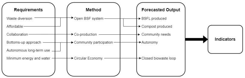
Biowaste management poses a significant and widespread challenge. However, its consideration as a resource has led to the emergence of innovative and sustainable biowaste management techniques. One such promising solution is the use of black soldier flies (BSF) in biowaste treatment. This technique offers various advantages, such as the transformation of biowaste into versatile products that can be used in agriculture, horticulture, aquaculture, animal husbandry, pharmaceuticals and energy production. Despite significant research on different aspects of the BSF biowaste treatment system, none have explored the application of circular economy principles in low-income settings using naturally occurring BSF, i.e., free-range BSF. This article addresses the gap utilizing a mixed-method approach through a case study to achieve two objectives: the localization of the circular economy through co-production with a community group and the viable production of black soldier fly larvae (BSFL) and compost to meet the community's needs. Through collaboration, a successful circular economy was established as biowaste was transformed into products and safely reintroduced into the local biosphere. Performance indices used included BSFL nutritional composition, harvest rates and heavy metal absence.
Through community involvement, circular economy principles were effectively implemented to redirect a retail market's fruit and vegetable waste from the landfill. The free-range open system produced 19.15 kg of BSFL, with 44.34% protein content, 20.6% crude fat and zero heavy metals. These outcomes align with existing research, indicating that a community-led open BSFL system can generate valuable products while fostering circular economy principles with minimal financial, technological, energy and water resources.
Citation: Atinuke Chineme, Getachew Assefa, Irene M. Herremans, Barry Wylant, Marwa Shumo, Aliceanna Shoo, Mturi James, Frida Ngalesoni, Anthony Ndjovu, Steve Mbuligwe, Mike Yhedgo. Advancing circular economy principles through wild black soldier flies[J]. AIMS Environmental Science, 2023, 10(6): 868-893. doi: 10.3934/environsci.2023047
Biowaste management poses a significant and widespread challenge. However, its consideration as a resource has led to the emergence of innovative and sustainable biowaste management techniques. One such promising solution is the use of black soldier flies (BSF) in biowaste treatment. This technique offers various advantages, such as the transformation of biowaste into versatile products that can be used in agriculture, horticulture, aquaculture, animal husbandry, pharmaceuticals and energy production. Despite significant research on different aspects of the BSF biowaste treatment system, none have explored the application of circular economy principles in low-income settings using naturally occurring BSF, i.e., free-range BSF. This article addresses the gap utilizing a mixed-method approach through a case study to achieve two objectives: the localization of the circular economy through co-production with a community group and the viable production of black soldier fly larvae (BSFL) and compost to meet the community's needs. Through collaboration, a successful circular economy was established as biowaste was transformed into products and safely reintroduced into the local biosphere. Performance indices used included BSFL nutritional composition, harvest rates and heavy metal absence.
Through community involvement, circular economy principles were effectively implemented to redirect a retail market's fruit and vegetable waste from the landfill. The free-range open system produced 19.15 kg of BSFL, with 44.34% protein content, 20.6% crude fat and zero heavy metals. These outcomes align with existing research, indicating that a community-led open BSFL system can generate valuable products while fostering circular economy principles with minimal financial, technological, energy and water resources.

| [1] | Kaza S, Yao L, Bhada-Tata P, Van Woerden F. What a Waste 2.0: A Global Snapshot of Solid Waste Management to 2050. Washington, DC: The World Bank; 2018. Available from: https://datatopics.worldbank.org/what-a-waste/trends_in_solid_waste_management.html https://doi.org/10.1596/978-1-4648-1329-0 |
| [2] | Jayasinghe R, Mushtaq U, Smythe TA, Baillie C, (2013) The Garbage Crisis: A Global Challenge for Engineers. San Rafael: Morgan & Claypool Publishers; 2013[cited 2021 Feb 17]. 3-5. https://www-morganclaypool-com.ezproxy.lib.ucalgary.ca/doi/pdfplus/10.2200/S00453ED1V01Y201301ETS018 |
| [3] | Ajibade LT (2007) Indigenous Knowledge System of waste management in Nigeria. IJTK 6: 642-647. |
| [4] |
Sridhar MKC, Hammed T (2014) Turning Waste to Wealth in Nigeria: An Overview. J Hum Ecol 46: 195–203. https://doi.org/10.1080/09709274.2014.11906720 doi: 10.1080/09709274.2014.11906720

|
| [5] |
Lohri CR, Diener S, Zabaleta I, Mertenat A, Zurbrügg C (2017) Treatment technologies for urban solid biowaste to create value products: a review with focus on low- and middle-income settings. Rev Environ Sci Biotechnol. 16: 81–130. https://doi.org/10.1007/s11157-017-9422-5 doi: 10.1007/s11157-017-9422-5
|
| [6] |
Asomani-Boateng R (2007) Closing the Loop: Community-Based Organic Solid Waste Recycling, Urban Gardening, and Land Use Planning in Ghana, West Africa. J Plan Educ Res 27: 132–45. https://doi.org/10.1177/0739456X07306392 doi: 10.1177/0739456X07306392
|
| [7] |
Asomani-Boateng R (2016) Local Networks: Commodity Queens and the Management of Organic Solid Waste in Indigenous Open-Air Markets in Accra, Ghana. J Plan Educ Res 36: 182–94. https://doi.org/10.1177/0739456X15604445 doi: 10.1177/0739456X15604445
|
| [8] | Dortmans B, Diener S, Verstappen B, Zurbrügg C.EAWAG in Switzerland: Black Soldier Fly Biowaste Processing. A Step-by-Step Guide. EAWAG – Swiss Federal Institute of Aquatic Science and Technology, 2017. Available from: https://www.eawag.ch/fileadmin/Domain1/Abteilungen/sandec/publikationen/SWM/BSF/BSF_Biowaste_Processing_HR.pdf |
| [9] | Edmond C. World Economic Forum in USA: This is what the world's waste does to people in poorer countries. World Economic Forum, 2019. Available from: https://www.weforum.org/agenda/2019/05/this-is-what-the-world-s-waste-does-to-people-in-poorer-countries/ |
| [10] |
Gahana GC, Patil YB, Shibin KT, et al. (2018) Conceptual frameworks for the drivers and barriers of integrated sustainable solid waste management: A TISM approach. Manag Environ Qual 29: 516–46. http://dx.doi.org.ezproxy.lib.ucalgary.ca/10.1108/MEQ-10-2017-0117 doi: 10.1108/MEQ-10-2017-0117
|
| [11] |
Oteng-Ababio M, Melara Arguello JE, Gabbay O (2013) Solid waste management in African cities: Sorting the facts from the fads in Accra, Ghana. Habitat Int 39: 96–104. https://doi.org/10.1016/j.habitatint.2012.10.010 doi: 10.1016/j.habitatint.2012.10.010
|
| [12] |
Siragusa L, Arzyutov D (2020) Nothing goes to waste: sustainable practices of re-use among Indigenous groups in the Russian North. Curr Opin Environ Sust 43 :41–8. https://doi.org/10.1016/j.cosust.2020.02.001 doi: 10.1016/j.cosust.2020.02.001
|
| [13] |
Cappellozza S, Leonardi MG, Savoldelli S, et al. (2019) A First Attempt to Produce Proteins from Insects by Means of a Circular Economy. Animals 9:278. https://doi.org/10.3390/ani9050278 doi: 10.3390/ani9050278
|
| [14] |
Shumo M, Osuga IM, Khamis FM, et al. (2019) The nutritive value of black soldier fly larvae reared on common organic waste streams in Kenya. Sci Rep 9: 10110. https://doi.org/10.1038/s41598-019-46603-z doi: 10.1038/s41598-019-46603-z
|
| [15] |
da Silva GDP, Hesselberg T (2020) A Review of the Use of Black Soldier Fly Larvae, Hermetia illucens (Diptera: Stratiomyidae), to Compost Organic Waste in Tropical Regions. Neotrop Entomol. 49: 151–62. https://doi.org/10.1007/s13744-019-00719-z doi: 10.1007/s13744-019-00719-z
|
| [16] |
Singh A, Kumari K (2019) An inclusive approach for organic waste treatment and valorisation using Black Soldier Fly larvae: A review. J Environ Manag 251: 109569. https://doi.org/10.1016/j.jenvman.2019.109569 doi: 10.1016/j.jenvman.2019.109569
|
| [17] |
Nyakeri EM, Ogola HJ, Ayieko MA (2017) An Open System for Farming Black Soldier Fly Larvae as a Source of Proteins for Smallscale Poultry and Fish Production. J Insects Food Feed 3: 51–56. https://doi.org/10.3920/JIFF2016.0030 doi: 10.3920/JIFF2016.0030
|
| [18] | Caplin R. Smith School of Enterprise and the Environment in University of Oxford; Business Models in Sustainability Transitions: A Study of Organic Waste Management and Black Soldier Fly Production in Kenya. Smith School of Enterprise and the Environment, Oxford, United Kingdom: Available from: https://www.linkedin.com/posts/ryancaplin_business-models-for-organic-waste-and-bsf-activity-6988508871459766272--5KL/ |
| [19] |
Ojha S, Bußler S, Schlüter OK (2020) Food waste valorisation and circular economy concepts in insect production and processing. Waste Manage 118: 600–9. https://doi.org/10.1016/j.wasman.2020.09.010 doi: 10.1016/j.wasman.2020.09.010
|
| [20] |
Gold M, Ireri D, Zurbrügg C, et al. (2021) Efficient and safe substrates for black soldier fly biowaste treatment along circular economy principles. Detritus 16: 31–40. https://doi.org/10.31025/2611-4135/2021.15116 doi: 10.31025/2611-4135/2021.15116
|
| [21] |
Paes LAB, Bezerra BS, Deus RM, et al. (2019) Organic solid waste management in a circular economy perspective – A systematic review and SWOT analysis. J Clean Prod 239: 118086. https://doi.org/10.1016/j.jclepro.2019.118086 doi: 10.1016/j.jclepro.2019.118086
|
| [22] |
Wang YS, Shelomi M (2017) Review of Black Soldier Fly (Hermetia illucens) as Animal Feed and Human Food. Foods 6:91. https://doi.org/10.3390/foods6100091 doi: 10.3390/foods6100091
|
| [23] |
Diener S, Zurbrügg C, Tockner K (2009) Conversion of organic material by black soldier fly larvae: establishing optimal feeding rates. Waste Manag Res. 27: 603–10. https://doi.org/10.1177/0734242X09103838 doi: 10.1177/0734242X09103838
|
| [24] |
Surendra KC, Tomberlin JK, van Huis A, et al. (2020) Rethinking organic wastes bioconversion: Evaluating the potential of the black soldier fly (Hermetia illucens (L.)) (Diptera: Stratiomyidae) (BSF). Waste Manage 117: 58–80. https://doi.org/10.1016/j.wasman.2020.07.050 doi: 10.1016/j.wasman.2020.07.050
|
| [25] | Diener S, Gutiérrez FR, Zurbrügg C, et al.Are Larvae of the Black Soldier Fly– Hermatia Illucens – A Financially Viable Option For Organic Waste Management in Costa Rica? In: Proceedings Sardinia 2009, Twelfth International Waste Management and Landfill Symposium. S. Margherita di Pula, Cagliari, Italy: CISA Publisher, Italy; 2009. |
| [26] | Diener S, Zurbrügg C, Gutiérrez FR, et al. WasteSafe in Khulna, Bangladesh: Black Soldier Fly Larvae For Organic Waste Treatment – Prospects And Constraints.; WasteSafe Khulna, Bangladesh, 2011 Available from: https://www.eawag.ch/fileadmin/Domain1/Abteilungen/sandec/publikationen/SWM/BSF/Black_soldier_fly_larvae_for_organic_waste_treatment.pdf |
| [27] |
Myers H, Tomberlin J, Lambert B, et al. (2008) Development of Black Soldier Fly (Diptera: Stratiomyidae) Larvae Fed Dairy Manure. Environ Entomol 37: 11–5. https://doi.org/10.1603/0046-225X(2008)37[11:DOBSFD]2.0.CO; 2 doi: 10.1093/ee/37.1.11
|
| [28] |
Isibika A, Simha P, Vinnerås B, et al. (2023) Food industry waste - An opportunity for black soldier fly larvae protein production in Tanzania. Sci Total Environ 858: 9. https://doi.org/10.1016/j.scitotenv.2022.159985 doi: 10.1016/j.scitotenv.2022.159985
|
| [29] |
Fuss M, Vasconcelos Barros RT, et al. (2018) Designing a framework for municipal solid waste management towards sustainability in emerging economy countries - An application to a case study in Belo Horizonte (Brazil). J Clean Prod 178: 655–64. https://doi.org/10.1016/j.jclepro.2018.01.051 doi: 10.1016/j.jclepro.2018.01.051
|
| [30] |
Yhdego M (1995) Urban solid waste management in Tanzania issues, concepts and challenges. Resources, Conserv Recy 14: 1–10. https://doi.org/10.1016/0921-3449(94)00017-Y doi: 10.1016/0921-3449(94)00017-Y
|
| [31] |
Ferronato N, Portillo MAG, Lizarazu GEG, et al. (2020) Formal and informal waste selective collection in developing megacities: Analysis of residents' involvement in Bolivia. Waste Manag Res. 39: 108–21. https://doi.org/10.1177/0734242X20936765 doi: 10.1177/0734242X20936765
|
| [32] |
Aleluia J, Ferrão P (2016) Characterization of urban waste management practices in developing Asian countries: A new analytical framework based on waste characteristics and urban dimension. Waste Manage 58: 415–29. https://doi.org/10.1016/j.wasman.2016.05.008 doi: 10.1016/j.wasman.2016.05.008
|
| [33] |
Ddiba D, Andersson K, Rosemarin A, et al. (2022) The circular economy potential of urban organic waste streams in low- and middle-income countries. Environ Dev Sustain. 24: 1116–44. https://doi.org/10.1007/s10668-021-01487-w doi: 10.1007/s10668-021-01487-w
|
| [34] |
Velenturf APM, Purnell P (2021) Principles for a sustainable circular economy. Sustain Prod Consump 27: 1437–57. https://doi.org/10.1016/j.spc.2021.02.018 doi: 10.1016/j.spc.2021.02.018
|
| [35] |
Suárez-Eiroa B, Fernández E, Méndez-Martínez G, et al. (2019) Operational principles of circular economy for sustainable development: Linking theory and practice. J Clean Prod 214: 952–61. https://doi.org/10.1016/j.jclepro.2018.12.271 doi: 10.1016/j.jclepro.2018.12.271
|
| [36] |
Wright CY, Godfrey L, Armiento G, et al. (2019) Circular economy and environmental health in low- and middle-income countries. Globalization Health 15: 65. https://doi.org/10.1186/s12992-019-0501-y doi: 10.1186/s12992-019-0501-y
|
| [37] |
Schroeder P, Dewick P, Kusi-Sarpong S, et al. (2018) Circular economy and power relations in global value chains: Tensions and trade-offs for lower income countries. Res Conserv Recy 136: 77–8. https://doi.org/10.1016/j.resconrec.2018.04.003 doi: 10.1016/j.resconrec.2018.04.003
|
| [38] |
Bringsken BM, Loureiro I, Ribeiro C, et al. (2018) Community Involvement Towards a Circular Economy: a Sociocultural Assessment of Projects and Interventions to Reduce Undifferentiated Waste. Eur J Sustain Dev 7: 496–506. https://doi.org/10.14207/ejsd.2018.v7n4p496 doi: 10.14207/ejsd.2018.v7n4p496
|
| [39] |
Padilla-Rivera A, do Carmo BBT, Arcese G, et al. (2021) Social circular economy indicators: Selection through fuzzy delphi method. Sustain Prod Consump 26: 101–110. https://doi.org/10.1016/j.spc.2020.09.015 doi: 10.1016/j.spc.2020.09.015
|
| [40] |
Chineme A, Assefa G, Herremans IM, et al. (2022) African Indigenous Female Entrepreneurs (IFÉs): A Closed-Looped Social Circular Economy Waste Management Model. Sustainability 14: 11628. https://doi.org/10.3390/su141811628 doi: 10.3390/su141811628
|
| [41] |
Ibáñez-Forés V, Bovea MD, Coutinho-Nóbrega C, et al. (2019) Assessing the social performance of municipal solid waste management systems in developing countries: Proposal of indicators and a case study. Ecol Indic 98: 164–178. https://doi.org/10.1016/j.ecolind.2018.10.031 doi: 10.1016/j.ecolind.2018.10.031
|
| [42] |
Verschuere B, Brandsen T, Pestoff V (2012) Co-production: The State of the Art in Research and the Future Agenda. VOLUNTAS: Int J Voluntary Nonprofit Org 23: 1083–1101. https://doi.org/10.1007/s11266-012-9307-8 doi: 10.1007/s11266-012-9307-8
|
| [43] |
Manuel-Navarrete D, Buzinde C, Swanson T (2021) Fostering horizontal knowledge co-production with Indigenous people by leveraging researchers' transdisciplinary intentions. Ecol Soc 26:22. https://doi.org/10.5751/ES-12265-260222 doi: 10.5751/ES-12265-260222
|
| [44] | Medina M, WIDER in Helsinki, Finland: Solid wastes, Poverty and the Environment in Developing Country Cities: Challenges and Opportunities. WIDER Helsinki, Finland, 2010. Available from: http://hdl.handle.net/10419/54107 |
| [45] |
Pestoff V (2014) Collective Action and the Sustainability of Co-Production. Public Manag Rev 16: 383–401. https://doi.org/10.1080/14719037.2013.841460 doi: 10.1080/14719037.2013.841460
|
| [46] | Amref Health Africa Tanzania. A Baseline Survey To Establish A Reference For A Functional Social Enterprise Based On The Current Practices, Demand And Attitudes Towards Solid Waste Management At Household Level In Ilala Municipal Council. 2018. Unpublished report by MK Center |
| [47] |
Halog A, Anieke S (2021) A Review of Circular Economy Studies in Developed Countries and Its Potential Adoption in Developing Countries. Circ Econ Sust 1 :209–230. https://doi.org/10.1007/s43615-021-00017-0 doi: 10.1007/s43615-021-00017-0
|
| [48] |
Korhonen J, Honkasalo A, Seppälä J (2018) Circular Economy: The Concept and its Limitations. Ecol Econ 143: 37–46. https://doi.org/10.1016/j.ecolecon.2017.06.041 doi: 10.1016/j.ecolecon.2017.06.041
|
| [49] | Ellen MacArthur Foundation. Towards the Circular Economy Vol. 1: An Economic and Business Rationale for an Accelerated Transition. Ellen MacArthur Foundation; 2013. Available from: https://emf.thirdlight.com/link/x8ay372a3r11-k6775n/@/preview/1?o |
| [50] | Robinson S. Social Circular Economy: Opportunities for People Planet and Profit. Social Circular Economy, 2017. Available from: http://www.socialcirculareconomy.com/news |
| [51] |
Gharfalkar M, Court R, Campbell C, et al. (2015) Analysis of waste hierarchy in the European waste directive 2008/98/EC. Waste Manage 39: 305–313. https://doi.org/10.1016/j.wasman.2015.02.007 doi: 10.1016/j.wasman.2015.02.007
|
| [52] |
Oh J, Hettiarachchi H (2020) Collective Action in Waste Management: A Comparative Study of Recycling and Recovery Initiatives from Brazil, Indonesia, and Nigeria Using the Institutional Analysis and Development Framework. Recycling 5:4. https://doi.org/10.3390/recycling5010004 doi: 10.3390/recycling5010004
|
| [53] | World Health Organization, United Nations City in Denmark Circular economy and health: opportunities and risks. World Health Organization. Regional Office for Europe, 2018. Available from: https://apps.who.int/iris/handle/10665/342218 |
| [54] |
Guo H, Jiang C, Zhang Z, et al. (2021) Material flow analysis and life cycle assessment of food waste bioconversion by black soldier fly larvae (Hermetia illucens L.). Sci Total Environ 750: 141656. https://doi.org/10.1016/j.scitotenv.2020.141656 doi: 10.1016/j.scitotenv.2020.141656
|
| [55] |
Salomone R, Saija G, Mondello G, et al. (2017) Environmental impact of food waste bioconversion by insects: Application of Life Cycle Assessment to process using Hermetia illucens. J Clean Prod 140: 890–905. https://doi.org/10.1016/j.jclepro.2016.06.154 doi: 10.1016/j.jclepro.2016.06.154
|
| [56] |
Sankara F, Sankara F, Pousga S, et al. (2023) Optimization of Production Methods for Black Soldier Fly Larvae (Hermetia illucens L.) in Burkina Faso. Insects 14: 776. https://doi.org/10.3390/insects14090776 doi: 10.3390/insects14090776
|
| [57] | Chineme A, Shumo M, Assefa G, et al. (2023) Simple is Better When Appropriate: An Innovative Accessible Approach to Biowaste Treatment Using Wild Black Soldier Fly, In: Solid Waste Management - Recent Advances, New Trends and Applications[Working Title]: IntechOpen, . http://dx.doi.org/10.5772/intechopen.1002449. |
| [58] | Bowan PA, Ziblim SD. (2020) Households' Knowledge, Attitudes, and Practices towards Municipal Solid Waste Disposal. J Studies Soc Sci 19. |
| [59] | Hammed T, Sridhar M, Olaseha I (2011) Effect of Demographic Characteristics and Perceptions of Community Residents on Solid Waste Management Practices in Orita-Aperin, Ibadan, Nigeria. J Environ Syst 33: 187–199. |
| [60] | Pfiester M, Kaufman PE. University of Florida in USA: Drone fly, rat-tailed maggot - Eristalis tenax (Linnaeus). University of Florida, s 2009. Available from: https://entnemdept.ufl.edu/creatures/livestock/rat-tailed_maggot.htm |
| [61] |
Ibrahim IA, Gad AM (1975) The Occurrence of Paedogenesis in Eristalis Larvae (Diptera: Syrphidae). J Med Entomol 12: 268. https://doi.org/10.1093/jmedent/12.2.268 doi: 10.1093/jmedent/12.2.268
|
| [62] | Alvarez L. The Role of Black Soldier Fly, Hermetia illucens (L.) (Diptera: Stratiomyidae) in Sustainable Waste Management in Northern Climates[Ph.D thesis].[Windsor]: University of Windsor; 2012. 171 p. |
| [63] |
Liu X, Chen X, Wang H, et al. (2017) Dynamic changes of nutrient composition throughout the entire life cycle of black soldier fly. PLOS ONE 2017 12: e0182601. https://doi.org/10.1371/journal.pone.0182601 doi: 10.1371/journal.pone.0182601
|


Figures(11) / Tables(4)

Atinuke Chineme, Getachew Assefa, Irene M. Herremans, Barry Wylant, Marwa Shumo, Aliceanna Shoo, Mturi James, Frida Ngalesoni, Anthony Ndjovu, Steve Mbuligwe, Mike Yhedgo. Advancing circular economy principles through wild black soldier flies[J]. AIMS Environmental Science, 2023, 10(6): 868-893. doi: 10.3934/environsci.2023047


 DownLoad: