Impact of antibody-level on viral shedding in B.1.617.2 (Delta) variant-infected patients analyzed using a joint model of longitudinal and time-to-event data

Yi Yin; Ting Zeng; Miao Lai; Zemin Luan; Kai Wang; Yuhang Ma; Zhiliang Hu; Kai Wang; Zhihang Peng; Yi Yin; Ting Zeng; Miao Lai; Zemin Luan; Kai Wang; Yuhang Ma; Zhiliang Hu; Kai Wang; Zhihang Peng

doi:10.3934/mbe.2023390

Mathematical Biosciences and Engineering

2023, Volume 20, Issue 5: 8875-8891. doi: 10.3934/mbe.2023390

Previous Article Next Article

Research article Special Issues

Impact of antibody-level on viral shedding in B.1.617.2 (Delta) variant-infected patients analyzed using a joint model of longitudinal and time-to-event data

1.
School of Public Health, Nanjing Medical University, Nanjing 211166, China
2.
College of Public Health, Xinjiang Medical University, Urumqi 830017, China
3.
Department of Medical Engineering and Technology, Xinjiang Medical University, Urumqi 830017, China
4.
Jiangsu Provincial Key Laboratory of Geriatrics, Department of Geriatrics, The First Affiliated Hospital of Nanjing Medical University, Nanjing 211166, China
5.
Department of Infectious Disease, the Second Hospital of Nanjing, Nanjing University of Chinese Medicine, Nanjing 210003, China
6.
Center for Global Health, School of Public Health, Nanjing Medical University, Nanjing 211166, China
^† These authors have contributed equally to this work

Received: 04 November 2022 Revised: 17 February 2023 Accepted: 27 February 2023 Published: 09 March 2023

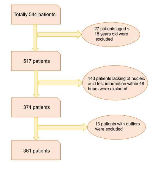
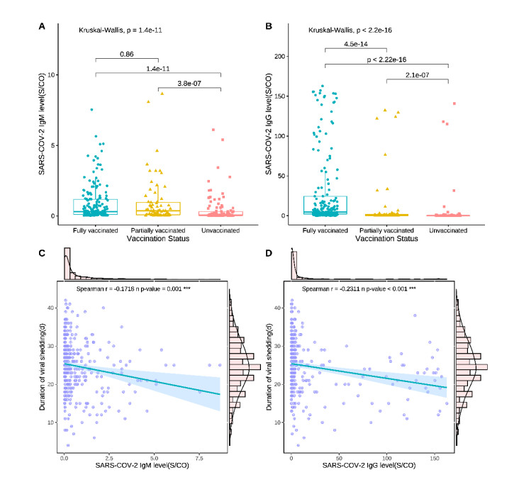
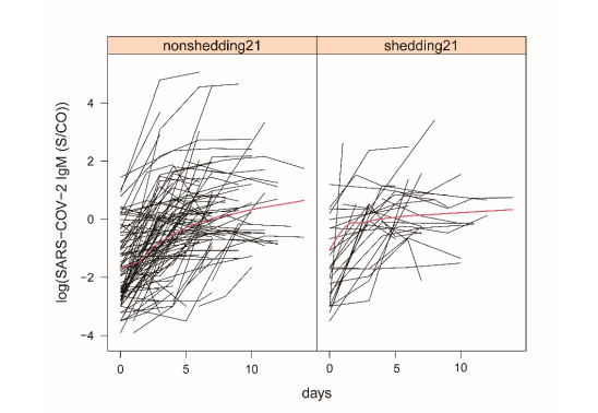
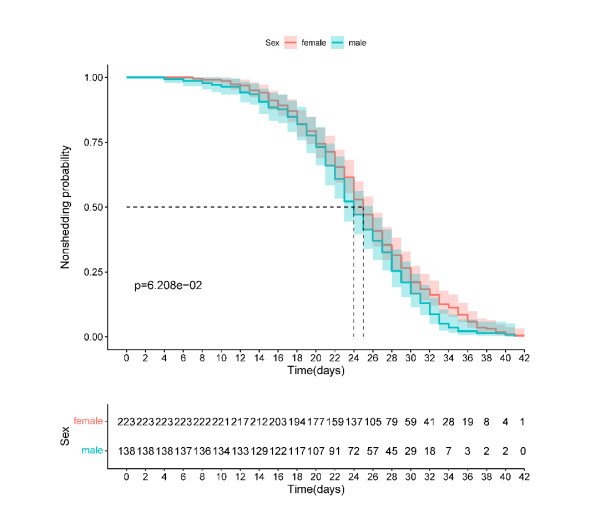
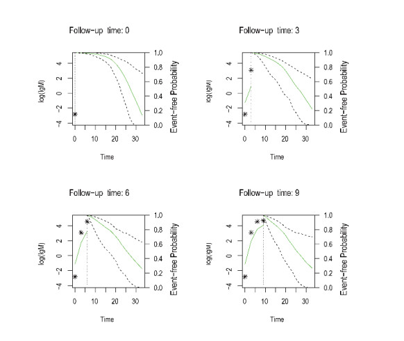
Knowledge of viral shedding remains limited. Repeated measurement data have been rarely used to explore the influencing factors. In this study, a joint model was developed to explore and validate the factors influencing the duration of viral shedding based on longitudinal data and survival data. We divided 361 patients infected with Delta variant hospitalized in Nanjing Second Hospital into two groups (≤ 21 days group and > 21 days group) according to the duration of viral shedding, and compared their baseline characteristics. Correlation analysis was performed to identify the factors influencing the duration of viral shedding. Further, a joint model was established based on longitudinal data and survival data, and the Markov chain Monte Carlo algorithm was used to explain the influencing factors. In correlation analysis, patients having received vaccination had a higher antibody level at admission than unvaccinated patients, and with the increase of antibody level, the duration of viral shedding shortened. The linear mixed-effects model showed the longitudinal variation of logSARS-COV-2 IgM sample/cutoff (S/CO) values, with a parameter estimate of 0.193 and a standard error of 0.017. Considering gender as an influencing factor, the parameter estimate of the Cox model and their standard error were 0.205 and 0.1093 (P = 0.608), the corresponding OR value was 1.228. The joint model output showed that SARS-COV-2 IgM (S/CO) level was strongly associated with the risk of a composite event at the 95% confidence level, and a doubling of SARS-COV-2 IgM (S/CO) level was associated with a 1.38-fold (95% CI: [1.16, 1.72]) increase in the risk of viral non-shedding. A higher antibody level in vaccinated patients, as well as the presence of IgM antibodies in serum, can accelerate shedding of the mutant virus. This study provides some evidence support for vaccine prevention and control of COVID-19 variants.
- COVID-19,
- SARS-CoV-2,
- viral shedding,
- joint model,
- antibodies
Citation: Yi Yin, Ting Zeng, Miao Lai, Zemin Luan, Kai Wang, Yuhang Ma, Zhiliang Hu, Kai Wang, Zhihang Peng. Impact of antibody-level on viral shedding in B.1.617.2 (Delta) variant-infected patients analyzed using a joint model of longitudinal and time-to-event data[J]. Mathematical Biosciences and Engineering, 2023, 20(5): 8875-8891. doi: 10.3934/mbe.2023390

Related Papers:

Abstract

Knowledge of viral shedding remains limited. Repeated measurement data have been rarely used to explore the influencing factors. In this study, a joint model was developed to explore and validate the factors influencing the duration of viral shedding based on longitudinal data and survival data. We divided 361 patients infected with Delta variant hospitalized in Nanjing Second Hospital into two groups (≤ 21 days group and > 21 days group) according to the duration of viral shedding, and compared their baseline characteristics. Correlation analysis was performed to identify the factors influencing the duration of viral shedding. Further, a joint model was established based on longitudinal data and survival data, and the Markov chain Monte Carlo algorithm was used to explain the influencing factors. In correlation analysis, patients having received vaccination had a higher antibody level at admission than unvaccinated patients, and with the increase of antibody level, the duration of viral shedding shortened. The linear mixed-effects model showed the longitudinal variation of logSARS-COV-2 IgM sample/cutoff (S/CO) values, with a parameter estimate of 0.193 and a standard error of 0.017. Considering gender as an influencing factor, the parameter estimate of the Cox model and their standard error were 0.205 and 0.1093 (P = 0.608), the corresponding OR value was 1.228. The joint model output showed that SARS-COV-2 IgM (S/CO) level was strongly associated with the risk of a composite event at the 95% confidence level, and a doubling of SARS-COV-2 IgM (S/CO) level was associated with a 1.38-fold (95% CI: [1.16, 1.72]) increase in the risk of viral non-shedding. A higher antibody level in vaccinated patients, as well as the presence of IgM antibodies in serum, can accelerate shedding of the mutant virus. This study provides some evidence support for vaccine prevention and control of COVID-19 variants.

References

[1]	WHO, Global Tuberculosis Report 2021, 2021. Available from: https://www.who.int/publications/i/item/9789240037021
[2]	WHO, Coronavirus Disease (COVID-19) Pandemic, 2019. Available from: https://www.who.int/emergencies/diseases/novel-coronavirus-2019
[3]	D. Tian, Y. Sun, J. Zhou, Q. Ye, The global epidemic of the SARS-CoV-2 Delta variant, key spike mutations and immune escape, Front. Immunol., 12 (2021), 5001. https://doi.org/10.3389/fimmu.2021.751778 doi: 10.3389/fimmu.2021.751778
[4]	L. Bian, Q. Gao, F. Gao, Q. Wang, Q. He, X. Wu, et al., Impact of the Delta variant on vaccine efficacy and response strategies, Expert Rev. Vaccines, 20 (2021), 1201–1209. https://10.1080/14760584.2021.1976153 doi: 10.1080/14760584.2021.1976153
[5]	S. Shiehzadegan, N. Alaghemand, M. Fox, V. Venketaraman, Analysis of the Delta Variant B.1.617.2 COVID-19, Clin. Pract., 11 (2021), 778–784. https://doi.org/10.3390/clinpract11040093 doi: 10.3390/clinpract11040093
[6]	WHO, Tracking SARS-CoV-2 Variants, 2022. Available from: https://www.who.int/activities/tracking-SARS-CoV-2-variants
[7]	V. T. Hoang, T. L. Dao, P. Gautret, Recurrence of positive SARS-CoV-2 in patients recovered from COVID-19, J. Med. Virol., 92 (2020), 2366–2367.
[8]	F. Zhou, T. Yu, R. Du, G. Fan, Y. Liu, Z. Liu, et al., Clinical course and risk factors for mortality of adult inpatients with COVID-19 in Wuhan, China: a retrospective cohort study, Lancet, 395 (2020), 1054–1062. https://10.1016/s0140-6736(20)30566-3
[9]	P. Y. Chia, S. W. X. Ong, C. J. Chiew, L. W. Ang, J. M. Chavatte, T. M. Mak, et al., Virological and serological kinetics of SARS-CoV-2 Delta variant vaccine breakthrough infections: A multicentre cohort study, Clin. Microbiol. Infec., 28 (2021). https://doi.org/10.1016/j.cmi.2021.11.010 doi: 10.1016/j.cmi.2021.11.010
[10]	H. Kato, K. Miyakawa, N. Ohtake, H. Go, Y. Yamaoka, S. Yajima, et al., Antibody titers against the Alpha, Beta, Gamma, and Delta variants of SARS-CoV-2 induced by BNT162b2 vaccination measured using automated chemiluminescent enzyme immunoassay, J. Infect. Chemother., 28 (2022), 273–278. https://doi.org/10.1016/j.jiac.2021.11.021 doi: 10.1016/j.jiac.2021.11.021
[11]	D. S. Khoury, D. Cromer, A. Reynaldi, T. E. Schlub, A. K. Wheatley, J. A. Juno, et al., Neutralizing antibody levels are highly predictive of immune protection from symptomatic SARS-CoV-2 infection, Nat. Med., 27 (2021), 1205–1211. https://doi.org/10.1038/s41591-021-01377-8 doi: 10.1038/s41591-021-01377-8
[12]	Z. Fang, Y. Zhang, C. Hang, J. Ai, S. Li, W. Zhang, Comparisons of viral shedding time of SARS-CoV-2 of different samples in ICU and non-ICU patients, J. Infection, 81 (2020), 147–178. https://doi.org/10.1016/j.jinf.2020.03.013 doi: 10.1016/j.jinf.2020.03.013
[13]	Y. Wang, L. Zhang, L. Sang, F. Ye, S. Ruan, B. Zhong, et al., Kinetics of viral load and antibody response in relation to COVID-19 severity, J. Clin. Invest., 130 (2020), 5235–5244. https://doi.org/10.1172/JCI138759 doi: 10.1172/JCI138759
[14]	Y. Liu, L. M. Yan, L. Wan, T. X. Xiang, A. Le, J. M. Liu, et al., Viral dynamics in mild and severe cases of COVID-19, Lancet Infect. Dis., 20 (2020), 656–657. https://doi.org/10.1016/S1473-3099(20)30232-2 doi: 10.1016/S1473-3099(20)30232-2
[15]	Y. Fu, P. Han, R. Zhu, T. Bai, J. Yi, X. Zhao, et al., Risk factors for viral RNA shedding in COVID-19 patients, Eur. Respiratory J., 56 (2020), 2001190. https://doi.org/10.1183/13993003.01190-2020 doi: 10.1183/13993003.01190-2020
[16]	K. Xu, Y. Chen, J. Yuan, P. Yi, C. Ding, W. Wu, et al., Factors Associated With Prolonged Viral RNA Shedding in Patients with Coronavirus Disease 2019 (COVID-19), Clin. Infect. Dis., 71 (2020), 799–806. https://doi.org/10.1093/cid/ciaa351 doi: 10.1093/cid/ciaa351
[17]	A. Mondi, P. Lorenzini, C. Castilletti, R. Gagliardini, E. Lalle, A. Corpolongo, et al., Risk and predictive factors of prolonged viral RNA shedding in upper respiratory specimens in a large cohort of COVID-19 patients admitted to an Italian reference hospital, Int. J. Infect. Dis., 105 (2021), 532–539. https://doi.org/10.1016/j.ijid.2021.02.117 doi: 10.1016/j.ijid.2021.02.117
[18]	H. Long, J. Zhao, H. L. Zeng, Q. B. Lu, L. Q. Fang, Q. Wang, et al., Prolonged viral shedding of SARS-CoV-2 and related factors in symptomatic COVID-19 patients: a prospective study, BMC Infect. Dis., 21 (2021), 1282. https://doi.org/10.1186/s12879-021-07002-w doi: 10.1186/s12879-021-07002-w
[19]	J. Gong, H. Dong, D. K. Wang, F. E. Lu, Z. Y. Huang, K. Fang, et al., Characteristics of Viral Shedding in Respiratory Samples and Specific Antibodies Production in 564 COVID-19 Patients, Curr. Med. Sci., 41 (2021), 46–50. https://doi.org/10.1007/s11596-021-2316-3 doi: 10.1007/s11596-021-2316-3
[20]	R. Ke, P. P. Martinez, R. L. Smith, L. L. Gibson, C. J. Achenbach, S. McFall, et al., Longitudinal analysis of SARS-CoV-2 vaccine breakthrough infections reveal limited infectious virus shedding and restricted tissue distribution, Open Forum Infect. Dis., 9 (2022). https://doi.org/10.1093/ofid/ofac192 doi: 10.1093/ofid/ofac192
[21]	K. Li, S. Luo, Dynamic prediction of Alzheimer's disease progression using features of multiple longitudinal outcomes and time-to-event data, Stat. Med., 38 (2019), 4804–4818. https://doi.org/10.1002/sim.8334 doi: 10.1002/sim.8334
[22]	A. Thomas, G. K. Vishwakarma, A. Bhattacharjee, Joint modeling of longitudinal and time-to-event data on multivariate protein biomarkers, J. Comput. Appl. Math., 381 (2021), 113016. https://doi.org/10.1016/j.cam.2020.113016 doi: 10.1016/j.cam.2020.113016
[23]	D. Rizopoulos, The R Package JMbayes for Fitting Joint Models for Longitudinal and Time-to-Event Data using MCMC, preprient, arXiv: 1404.7625.
[24]	Y. L. Lee, C. H. Liao, P. Y. Liu, C. Y. Cheng, M. Y. Chung, C. E. Liu, et al., Dynamics of anti-SARS-Cov-2 IgM and IgG antibodies among COVID-19 patients, J. Infect., 81 (2020), e55–e58. https://doi.org/10.1016/j.jinf.2020.04.019 doi: 10.1016/j.jinf.2020.04.019
[25]	J. Shang, Y. Wan, C. Luo, G. Ye, Q. Geng, A. Auerbach, et al., Cell entry mechanisms of SARS-CoV-2, Proc. Natl. Acad. Sci. USA, 117 (2020), 11727–11734. https://doi.org/10.1073/pnas.2003138117 doi: 10.1073/pnas.2003138117
[26]	Z. Wang, F. Schmidt, Y. Weisblum, F. Muecksch, C. O. Barnes, S. Finkin, et al., mRNA vaccine-elicited antibodies to SARS-CoV-2 and circulating variants, Nature, 592 (2021), 616–622. https://doi.org/10.1038/s41586-021-03324-6 doi: 10.1038/s41586-021-03324-6
[27]	Y. Li, G. Wang, N. Li, Y. Wang, Q. Zhu, H. Chu, et al., Structural insights into immunoglobulin M, Science, 367 (2020), 1014–1017. https://doi.org/10.1126/science.aaz5425 doi: 10.1126/science.aaz5425
[28]	C. Gaebler, Z. Wang, J. C. C. Lorenzi, F. Muecksch, S. Finkin, M. Tokuyama, et al., Evolution of antibody immunity to SARS-CoV-2, Nature, 591 (2021), 639–644. https://doi.org/10.1038/s41586-021-03207-w doi: 10.1038/s41586-021-03207-w
[29]	J. Carrillo, N. Izquierdo-Useros, C. Ávila-Nieto, E. Pradenas, B. Clotet, J. Blanco, Humoral immune responses and neutralizing antibodies against SARS-CoV-2; implications in pathogenesis and protective immunity, Biochem. Biophs. Res. Commun., 538 (2021), 187–191. https://doi.org/10.1016/j.bbrc.2020.10.108 doi: 10.1016/j.bbrc.2020.10.108
[30]	M. A. Tortorici, M. Beltramello, F. A. Lempp, D. Pinto, H. V. Dang, L. E. Rosen, et al., Ultrapotent human antibodies protect against SARS-CoV-2 challenge via multiple mechanisms, Science, 370 (2020), 950–957. https://doi.org/10.1126/science.abe3354 doi: 10.1126/science.abe3354
[31]	Z. Ku, X. Xie, P. R. Hinton, X. Liu, X. Ye, A. E. Muruato, et al., Nasal delivery of an IgM offers broad protection from SARS-CoV-2 variants, Nature, 595 (2021), 718–723. https://doi.org/10.1038/s41586-021-03673-2 doi: 10.1038/s41586-021-03673-2
[32]	T. Fiolet, Y. Kherabi, C. J. MacDonald, J. Ghosn, N. Peiffer-Smadja, Comparing COVID-19 vaccines for their characteristics, efficacy and effectiveness against SARS-CoV-2 and variants of concern: A narrative review, Clin. Microbiol. Infect., 28 (2022), 202–221. https://doi.org/10.1016/j.cmi.2021.10.005 doi: 10.1016/j.cmi.2021.10.005
[33]	M. Levine-Tiefenbrun, I. Yelin, R. Katz, E. Herzel, Z. Golan, L. Schreiber, et al., Initial report of decreased SARS-CoV-2 viral load after inoculation with the BNT162b2 vaccine, Nat. Med., 27 (2021), 790–792. https://doi.org/10.1038/s41591-021-01316-7 doi: 10.1038/s41591-021-01316-7

Reader Comments

Your name:*

Email:*
© 2023 the Author(s), licensee AIMS Press. This is an open access article distributed under the terms of the Creative Commons Attribution License (http://creativecommons.org/licenses/by/4.0)