A double-channel multiscale depthwise separable convolutional neural network for abnormal gait recognition

Xiaoguang Liu; Yubo Wu; Meng Chen; Tie Liang; Fei Han; Xiuling Liu; Xiaoguang Liu; Yubo Wu; Meng Chen; Tie Liang; Fei Han; Xiuling Liu

doi:10.3934/mbe.2023349

Mathematical Biosciences and Engineering

2023, Volume 20, Issue 5: 8049-8067. doi: 10.3934/mbe.2023349

Previous Article Next Article

Research article

A double-channel multiscale depthwise separable convolutional neural network for abnormal gait recognition

1.
College of Electronic and Information Engineering, Hebei University, Baoding, China
2.
Key Laboratory of Digital Medical Engineering of Hebei Province, Hebei University, Baoding, China

Academic Editor: Hao Wang

Received: 15 January 2023 Revised: 07 February 2023 Accepted: 13 February 2023 Published: 23 February 2023

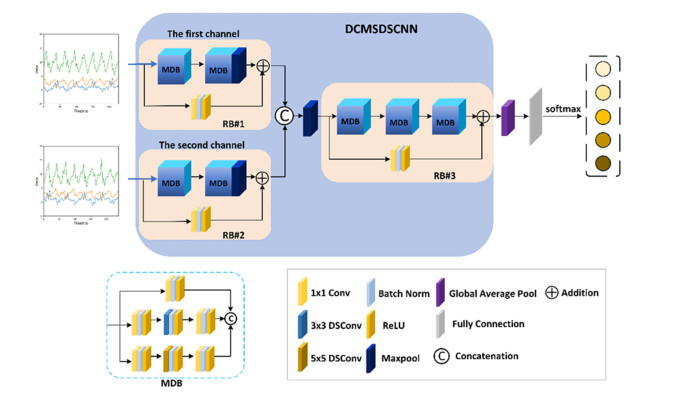
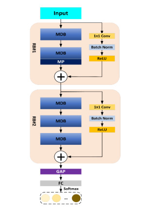
Abnormal gait recognition is important for detecting body part weakness and diagnosing diseases. The abnormal gait hides a considerable amount of information. In order to extract the fine, spatial feature information in the abnormal gait and reduce the computational cost arising from excessive network parameters, this paper proposes a double-channel multiscale depthwise separable convolutional neural network (DCMSDSCNN) for abnormal gait recognition. The method designs a multiscale depthwise feature extraction block (MDB), uses depthwise separable convolution (DSC) instead of standard convolution in the module and introduces the Bottleneck (BK) structure to optimize the MDB. The module achieves the extraction of effective features of abnormal gaits at different scales, and reduces the computational cost of the network. Experimental results show that the gait recognition accuracy is up to 99.60%, while the memory size of the model is reduced 4.21 times than before optimization.
- abnormal gait recognition,
- convolutional neural network (CNN),
- MDB,
- BK structure,
- double-channel network
Citation: Xiaoguang Liu, Yubo Wu, Meng Chen, Tie Liang, Fei Han, Xiuling Liu. A double-channel multiscale depthwise separable convolutional neural network for abnormal gait recognition[J]. Mathematical Biosciences and Engineering, 2023, 20(5): 8049-8067. doi: 10.3934/mbe.2023349

Related Papers:

Abstract

Abnormal gait recognition is important for detecting body part weakness and diagnosing diseases. The abnormal gait hides a considerable amount of information. In order to extract the fine, spatial feature information in the abnormal gait and reduce the computational cost arising from excessive network parameters, this paper proposes a double-channel multiscale depthwise separable convolutional neural network (DCMSDSCNN) for abnormal gait recognition. The method designs a multiscale depthwise feature extraction block (MDB), uses depthwise separable convolution (DSC) instead of standard convolution in the module and introduces the Bottleneck (BK) structure to optimize the MDB. The module achieves the extraction of effective features of abnormal gaits at different scales, and reduces the computational cost of the network. Experimental results show that the gait recognition accuracy is up to 99.60%, while the memory size of the model is reduced 4.21 times than before optimization.

References

[1]	J. M. Hausdorff, D. A. Rios, H. K. Edelberg, Gait variability and fall risk in community-living older adults: A 1-year prospective study, Arch. Phys. Med. Rehabil., 82 (2001), 1050–1056. https://doi.org/10.1053/apmr.2001.24893 doi: 10.1053/apmr.2001.24893
[2]	S. Wu, J. Ou, L. Shu, G. Hu, Z. Song, X. Xu, et al., MhNet: Multi-scale spatio-temporal hierarchical network for real-time wearable fall risk assessment of the elderly, Comput. Biol. Med., 144 (2022), 105355. https://doi.org/10.1016/j.compbiomed.2022.105355 doi: 10.1016/j.compbiomed.2022.105355
[3]	I. Mileti, J. Taborri, S. Rossi, M. Petrarca, F. Patanè, P. Cappa, Evaluation of the effects on stride-to-stride variability and gait asymmetry in children with Cerebral Palsy wearing the WAKE-up ankle module, in 2016 IEEE International Symposium on Medical Measurements and Applications (MeMeA), (2016), 1–6. https://doi.org/ 10.1109/MeMeA.2016.7533748
[4]	H. C. Chang, Y. L. Hsu, S. C. Yang, J. C. Lin, Z. H. Wu, A wearable inertial measurement system with complementary filter for gait analysis of patients with stroke or Parkinson's disease, IEEE Access, 4 (2016), 8442–8453. https://doi.org/ 10.1109/ACCESS.2016.2633304
[5]	J. M. Hausdorff, M. E. Cudkowicz, R. Firtion, J. Y. Wei, A. L. Goldberger, Gait variability and basal ganglia disorders: stride‐to‐stride variations of gait cycle timing in Parkinson's disease and Huntington's disease, Mov. Disord., 13 (1998), 428–437. https://doi.org/10.1002/mds.870130310 doi: 10.1002/mds.870130310
[6]	T. N. Nguyen, H. H. Huynh, J. Meunier, Skeleton-based abnormal gait detection, Sensors, 16 (2016), 1792. https://doi.org/10.3390/s16111792 doi: 10.3390/s16111792
[7]	R. Rucco, V. Agosti, F. Jacini, P. Sorrentino, P. Varriale, M. de Stefano, et al., Spatio-temporal and kinematic gait analysis in patients with Frontotemporal dementia and Alzheimer's disease through 3D motion capture, Gait Posture 52 (2017), 312–317. https://doi.org/10.1016/j.gaitpost.2016.12.021 doi: 10.1016/j.gaitpost.2016.12.021
[8]	J. Jenkins, C. Ellis, Using ground reaction forces from gait analysis: Body mass as a weak biometric, in International Conference on Pervasive Computing, 4480 (2007), 251–267. https://doi.org/ 10.1007/978-3-540-72037-9_15
[9]	T. C. Pataky, T. Mu, K. Bosch, D. Rosenbaum, J. Y. Goulermas, Gait recognition: Highly unique dynamic plantar pressure patterns among 104 individuals, J. R. Soc., Interface, 9 (2012), 790–800. https://doi.org/10.1098/rsif.2011.0430 doi: 10.1098/rsif.2011.0430
[10]	A. Mannini, D. Trojaniello, A. Cereatti, A. M. Sabatini, A machine learning framework for gait classification using inertial sensors: Application to elderly, post-stroke and huntington's disease patients, Sensors, 16 (2016), 134. https://doi.org/ 10.3390/s16010134
[11]	M. Alaqtash, T. Sarkodie-Gyan, H. Yu, O. Fuentes, R. Brower, A. Abdelgawad, Automatic classification of pathological gait patterns using ground reaction forces and machine learning algorithms, in 2011 Annual International Conference of the IEEE Engineering in Medicine and Biology Society, (2011), 453–457. https://doi.org/ 10.1109/IEMBS.2011.6090063
[12]	N. Mezghani, S. Husse, K. Boivin, K. Turcot, R. Aissaoui, N. Hagemeister, et al., Automatic classification of asymptomatic and osteoarthritis knee gait patterns using kinematic data features and the nearest neighbor classifier, IEEE Trans. Biomed. Eng., 55 (2008), 1230–1232. https://doi.org/10.1109/TBME.2007.905388 doi: 10.1109/TBME.2007.905388
[13]	H. Guan-Wei, L. Min-Hsuan, C. Yu-Tai, Methods for person recognition and abnormal gait detection using tri-axial accelerometer and gyroscope, in 2017 International Conference on Computational Science and Computational Intelligence (CSCI), (2017), 1691–1694. https://doi.org/ 10.1109/CSCI.2017.294
[14]	Y. Bengio, A. Courville, P. Vincent, Representation learning: A review and new perspectives, IEEE Trans. Pattern Anal. Mach. Intell., 35 (2013), 1798–1828. https://doi.org/10.1109/TPAMI.2013.50 doi: 10.1109/TPAMI.2013.50
[15]	I. Huitzil, L. Dranca, J. Bernad, F. Bobillo, Gait recognition using fuzzy ontologies and Kinect sensor data, Int. J. Approx. Reason., 113 (2019), 354–371. https://doi.org/10.1016/j.ijar.2019.07.012 doi: 10.1016/j.ijar.2019.07.012
[16]	M. Gadaleta, L. Merelli, M. Rossi, Human authentication from ankle motion data using convolutional neural networks, in 2016 IEEE Statistical Signal Processing Workshop (SSP), (2016), 1–5. https://doi.org/ 10.1109/SSP.2016.7551815
[17]	J. Gao, P. Gu, Q. Ren, J. Zhang, X. Song, Abnormal gait recognition algorithm based on LSTM-CNN fusion network, IEEE Access, 7 (2019), 163180–163190. https://doi.org/10.1109/ACCESS.2019.2950254 doi: 10.1109/ACCESS.2019.2950254
[18]	J. Chakraborty, A. Nandy, Discrete wavelet transform based data representation in deep neural network for gait abnormality detection, Biomed. Signal Process. Control, 62 (2020), 102076. https://doi.org/10.1016/j.bspc.2020.102076 doi: 10.1016/j.bspc.2020.102076
[19]	K. Jun, S. Lee, D. W. Lee, M. S. Kim, Deep learning-based multimodal abnormal gait classification using a 3D skeleton and plantar foot pressure, IEEE Access, 9 (2021), 161576–161589. https://doi.org/10.1109/ACCESS.2021.3131613 doi: 10.1109/ACCESS.2021.3131613
[20]	K. He, X. Zhang, S. Ren, J. Sun, Deep residual learning for image recognition, in 2016 IEEE Conference on Computer Vision and Pattern Recognition (CVPR), (2016), 770–778. https://doi.org/ 10.1109/CVPR.2016.90
[21]	C. Szegedy, V. Vanhoucke, S. Ioffe, J. Shlens, Z. Wojna, Rethinking the inception architecture for computer vision, in 2016 IEEE Conference on Computer Vision and Pattern Recognition (CVPR), (2016), 2818–2826. https://doi.org/ 10.1109/CVPR.2016.308
[22]	S. Woo, J. Park, J. Y. Lee, I. S. Kweon, CBAM: Convolutional block attention module, in European Conference on Computer Vision, (2018), 3–19. https://doi.org/ 10.1007/978-3-030-01234-2_1
[23]	H. Huang, P. Zhou, Y. Li, F. Sun, A lightweight attention-based CNN model for efficient gait recognition with wearable IMU sensors, Sensors, 21 (2021), 2866. https://doi.org/10.3390/s21082866 doi: 10.3390/s21082866
[24]	K. He, X. Zhang, S. Ren, J. Sun, Identity mappings in deep residual networks, in European Conference on Computer Vision, (2016), 630–645. https://doi.org/ 10.1007/978-3-319-46493-0_38
[25]	M. Shafiq, Z. Gu, Deep residual learning for image recognition: A survey, Appl. Sci., 12 (2022), 8972. https://doi.org/10.3390/app12188972 doi: 10.3390/app12188972
[26]	M. Paulich, M. Schepers, N. Rudigkeit, G. Bellusci, Xsens MTw Awinda: Miniature wireless inertial-magnetic motion tracker for highly accurate 3D kinematic applications, XSens Technol., (2018), 1–9. https://doi.org/ 10.13140/RG.2.2.23576.49929
[27]	M. Musci, D. De Martini, N. Blago, T. Facchinetti, M. Piastra, Online fall detection using recurrent neural networks, preprint, arXiv: 1804.04976.
[28]	F. Chollet, Xception: Deep learning with depthwise separable convolutions, in 2017 IEEE Conference on Computer Vision and Pattern Recognition (CVPR), (2017), 1800–1807. https://doi.org/ 10.1109/CVPR.2017.195
[29]	W. Li, X. Zhang, Y. Peng, M. Dong, Spatiotemporal fusion of remote sensing images using a convolutional neural network with attention and multiscale mechanisms, Int. J. Remote Sens., 42 (2021), 1973–1993. https://doi.org/10.1080/01431161.2020.1809742 doi: 10.1080/01431161.2020.1809742
[30]	D. P. Kingma, J. Ba, Adam: A method for stochastic optimization, preprint, arXiv: 1412.6980.
[31]	A. Rohan, M. Rabah, T. Hosny, S. Kim, Human pose estimation-based real-time gait analysis using convolutional neural network, IEEE Access, 8 (2020), 191542–191550. https://doi.org/10.1109/ACCESS.2020.3030086 doi: 10.1109/ACCESS.2020.3030086
[32]	Q. Zou, Y. Wang, Q. Wang, Y. Zhao, Q. Li, Deep learning-based gait recognition using smartphones in the wild, IEEE Trans. Inf. Forensics Secur., 15 (2020), 3197–3212. https://doi.org/10.1109/TIFS.2020.2985628 doi: 10.1109/TIFS.2020.2985628
[33]	A. S. Alharthi, K. B. Ozanyan, Deep learning for ground reaction force data analysis: Application to wide-area floor sensing, in 2019 IEEE 28th International Symposium on Industrial Electronics (ISIE), (2019), 1401–1406. https://doi.org/ 10.1109/ISIE.2019.8781511
[34]	Y. Zhao, J. Li, X. Wang, F. Liu, P. Shan, L. Li, et al., A lightweight pose sensing scheme for contactless abnormal gait behavior measurement, Sensors, 22 (2022), 4070. https://doi.org/10.3390/s22114070 doi: 10.3390/s22114070

Reader Comments

Your name:*

Email:*
© 2023 the Author(s), licensee AIMS Press. This is an open access article distributed under the terms of the Creative Commons Attribution License (http://creativecommons.org/licenses/by/4.0)