Propagation dynamics in an SIRS model with general incidence functions

Wenhao Chen; Guo Lin; Shuxia Pan; Wenhao Chen; Guo Lin; Shuxia Pan

doi:10.3934/mbe.2023291

Mathematical Biosciences and Engineering

2023, Volume 20, Issue 4: 6751-6775. doi: 10.3934/mbe.2023291

Previous Article Next Article

Research article Special Issues

Propagation dynamics in an SIRS model with general incidence functions

1.
School of Mathematics and Statistics, Lanzhou University, Lanzhou 730000, Gansu, China
2.
School of Science, Lanzhou University of Technology, Lanzhou 730050, Gansu, China

Academic Editor: Xiang-Sheng Wang

Received: 26 December 2022 Revised: 27 January 2023 Accepted: 28 January 2023 Published: 06 February 2023

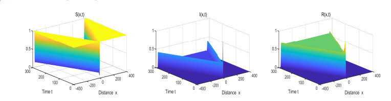
This paper studies the initial value problems and traveling wave solutions in an SIRS model with general incidence functions. Linearizing the infected equation at the disease free steady state, we can define a threshold if the corresponding basic reproduction ratio in kinetic system is larger than the unit. When the initial condition for the infected is compactly supported, we prove that the threshold is the spreading speed for three unknown functions. At the same time, this threshold is the minimal wave speed for traveling wave solutions modeling the disease spreading process. If the corresponding basic reproduction ratio in kinetic system is smaller than the unit, then we confirm the extinction of the infected and the nonexistence of nonconstant traveling waves.
- comparison principle,
- upper and lower solutions,
- asymptotic spreading,
- minimal wave speed,
- spreading speed
Citation: Wenhao Chen, Guo Lin, Shuxia Pan. Propagation dynamics in an SIRS model with general incidence functions[J]. Mathematical Biosciences and Engineering, 2023, 20(4): 6751-6775. doi: 10.3934/mbe.2023291

Related Papers:

Abstract

This paper studies the initial value problems and traveling wave solutions in an SIRS model with general incidence functions. Linearizing the infected equation at the disease free steady state, we can define a threshold if the corresponding basic reproduction ratio in kinetic system is larger than the unit. When the initial condition for the infected is compactly supported, we prove that the threshold is the spreading speed for three unknown functions. At the same time, this threshold is the minimal wave speed for traveling wave solutions modeling the disease spreading process. If the corresponding basic reproduction ratio in kinetic system is smaller than the unit, then we confirm the extinction of the infected and the nonexistence of nonconstant traveling waves.

References

[1]	W. O. Kermack, A. G. McKendrick, A contribution to the mathematical theory of epidemics, in Proceedings of the Royal Society of London. Series A, Containing Papers of A Mathematical and Physical Character, 115 (1927), 700–721. https://doi.org/10.1098/rspa.1927.0118
[2]	Q. Pan, J. Huang, H. Wang, An SIRS model with nonmonotone incidence and saturated treatment in a changing environment, J. Math. Biol., 85 (2022), 23. https://doi.org/10.1007/s00285-022-01787-3 doi: 10.1007/s00285-022-01787-3
[3]	J. D. Murray, Mathematical Biology II: Spatial Models and Biomedical Applications, 3rd edition, Springer-Verlag, New York, 2003. https://doi.org/10.1007/b98869
[4]	L. Rass, J. Radcliffe, Spatial Deterministic Epidemics, AMS, Providence, RI, 2003. https://doi.org/10.1090/surv/102
[5]	S. Ruan, Spatial-temporal dynamics in nonlocal epidemiological models, in Mathematics for Life Science and Medicine (eds. Y. Takeuchi, K. Sato, Y. Iwasa), Springer-Verlag, New York, (2007), 97–122. https://doi.org/10.1007/978-3-540-34426-1_5
[6]	E. Avila-Vales, A. G. C. Perez, Dynamics of a reaction-diffusion SIRS model with general incidence rate in a heterogeneous environment, Z. Angew. Math. Phys., 73 (2022), 9. https://doi.org/10.1007/s00033-021-01645-0 doi: 10.1007/s00033-021-01645-0
[7]	D. G. Aronson, H. F. Weinberger, Nonlinear diffusion in population genetics, combustion, and nerve pulse propagation, in Partial Differential Equations and Related Topics, Springer Berlin Heidelberg, Berlin, Heidelberg, (1975), 5–49. https://doi.org/10.1007/BFb0070595
[8]	R. A. Fisher, The wave of advance of advantageous genes, Ann. Eugen., 7 (1937), 355–369. https://doi.org/10.1111/j.1469-1809.1937.tb02153.x doi: 10.1111/j.1469-1809.1937.tb02153.x
[9]	A. N. Kolmogorov, I. G. Petrovskii, N. S. Piskunov, Study of a diffusion equation that is related to the growth of a quality of matter, and its application to a biological problem, Byul. Mosk. Gos. Univ. Ser. A: Mat. Mekh., 1 (1937), 1–26.
[10]	K. J. Brown, J. Carr, Deterministic epidemic waves of critical velocity, in Mathematical Proceedings of the Cambridge Philosophical Society, 81 (1977), 431–433. https://doi.org/10.1017/S0305004100053494
[11]	O. Diekmann, Thresholds and travelling waves for the geographical spread of infection, J. Math. Biol., 6 (1978), 109–130. https://doi.org/10.1007/BF02450783 doi: 10.1007/BF02450783
[12]	O. Diekmann, Run for your life. A note on the asymptotic speed of propagation of an epidemic, J. Differ. Equations, 33 (1979), 58–73. https://doi.org/10.1016/0022-0396(79)90080-9 doi: 10.1016/0022-0396(79)90080-9
[13]	H. R. Thieme, A model for the spatial spread of an epidemic, J. Math. Biol., 4 (1977), 337–351. https://doi.org/10.1007/BF00275082 doi: 10.1007/BF00275082
[14]	H. R. Thieme, Density-dependent regulation of spatially distributed populations and their asymptotic speed of spread, J. Math. Biol., 8 (1979), 173–187. https://doi.org/10.1007/BF00279720 doi: 10.1007/BF00279720
[15]	H. F. Weinberger, M. A. Lewis, B. Li, Analysis of linear determinacy for spread in cooperative models, J. Math. Biol., 45 (2002), 183–218. https://doi.org/10.1007/s002850200145 doi: 10.1007/s002850200145
[16]	Q. Ye, Z. Li, M. Wang, Y. Wu, Introduction to Reaction Diffusion Equations, 2nd edition, Science Press, Beijing, 2011.
[17]	H. L. Smith, Monotone Dynamical Systems: An Introduction to the Theory of Competitive and Cooperative Systems, AMS, Providence, RI, 1995. https://doi.org/10.1090/surv/041
[18]	G. Nadin, L. Rossi, Propagation phenomena for time heterogeneous KPP reaction-diffusion equations, J. Math. Pures Appl., 98 (2012), 633–653. https://doi.org/10.1016/j.matpur.2012.05.005 doi: 10.1016/j.matpur.2012.05.005
[19]	L. Rossi, The Freidlin-Gärtner formula for general reaction terms, Adv. Math., 317 (2017), 267–298. https://doi.org/10.1016/j.aim.2017.07.002 doi: 10.1016/j.aim.2017.07.002
[20]	A. Ducrot, Spatial propagation for a two component reaction-diffusion system arising in population dynamics, J. Differ. Equations, 260 (2016), 8316–8357. https://doi.org/10.1016/j.jde.2016.02.023 doi: 10.1016/j.jde.2016.02.023
[21]	X. Wang, G. Lin, S. Ruan, Spreading speeds and traveling wave solutions of diffusive vector-borne disease models without monotonicity, Proc. Roy. Soc. Edinburgh Sect. A, 2021 (2021), 1–30. https://doi.org/10.1017/prm.2021.76 doi: 10.1017/prm.2021.76
[22]	R. L. Abi, J. B. Burie, A. Ducrot, Asymptotic speed of spread for a nonlocal evolutionary-epidemic system, Discrete Contin. Dyn. Syst., 41 (2021), 4959–4985. https://doi.org/10.3934/dcds.2021064 doi: 10.3934/dcds.2021064
[23]	X. Chen, J. C. Tsai, Spreading speed in a farmers and hunter-gatherers model arising from Neolithic transition in Europe, J. Math. Pures Appl., 143 (2020), 192–207. https://doi.org/10.1016/j.matpur.2020.03.007 doi: 10.1016/j.matpur.2020.03.007
[24]	A. Ducrot, T. Giletti, J. S. Guo, M. Shimojo, Asymptotic spreading speeds for predator-prey system with two predators and one prey, Nonlinearity, 34 (2021), 669–704. https://doi.org/10.1088/1361-6544/abd289 doi: 10.1088/1361-6544/abd289
[25]	S. L. Wu, L. Pang, S. Ruan, Propagation dynamics in periodic predator-prey systems with nonlocal dispersal, J. Math. Pures Appl., 170 (2023), 57–95. https://doi.org/10.1016/j.matpur.2022.12.003 doi: 10.1016/j.matpur.2022.12.003
[26]	D. Xiao, R. Mori, Spreading properties of a three-component reaction-diffusion model for the population of farmers and hunter-gatherers, Ann. Inst. H. Poincaré Anal. Non Linéaire, 38 (2021), 911–951. https://doi.org/10.1016/j.anihpc.2020.09.007
[27]	M. Zhao, R. Yuan, Z. Ma, X. Zhao, Spreading speeds for the predator-prey system with nonlocal dispersal, J. Differ. Equations, 316 (2022), 552–598. https://doi.org/10.1016/j.jde.2022.01.038 doi: 10.1016/j.jde.2022.01.038
[28]	J. Fang, X. Q. Zhao, Monotone wavefronts of the nonlocal Fisher-KPP equation, Nonlinearity, 24 (2011), 3043–3054. https://doi.org/10.1088/0951-7715/24/11/002 doi: 10.1088/0951-7715/24/11/002
[29]	M. Huang, S. L. Wu, X. Q. Zhao, Propagation dynamics for time-periodic and partially degenerate reaction-diffusion systems, SIAM J. Math. Anal., 54 (2022), 1860–1897. https://doi.org/10.1137/21M1397234 doi: 10.1137/21M1397234
[30]	X. Liang, X. Q. Zhao, Asymptotic speeds of spread and traveling waves for monotone semiflows with applications, Commun. Pure Appl. Math., 60 (2007), 1–40. https://doi.org/10.1002/cpa.20154 doi: 10.1002/cpa.20154
[31]	G. Lin, S. Ruan, Traveling wave solutions for delayed reaction-diffusion systems and applications to Lotka-Volterra competition-diffusion models with distributed delays, J. Dyn. Differ. Equations, 26 (2014), 583–605. https://doi.org/10.1007/s10884-014-9355-4 doi: 10.1007/s10884-014-9355-4
[32]	J. Huang, X. Zou, Existence of traveling wavefronts of delayed reaction-diffusion systems without monotonicity, Discrete Contin. Dyn. Syst., 9 (2003), 925–936. https://doi.org/10.3934/dcds.2003.9.925 doi: 10.3934/dcds.2003.9.925
[33]	S. Ma, Traveling wavefronts for delayed reaction-diffusion systems via a fixed point theorem, J. Differ. Equations, 171 (2001), 294–314. https://doi.org/10.1006/jdeq.2000.3846 doi: 10.1006/jdeq.2000.3846
[34]	W. J. Sheng, M. Wang, Z. C. Wang, Propagation phenomena in a diffusion system with the Belousov-Zhabotinskii chemical reaction, Commun. Contemp. Math., https://doi.org/10.1142/S0219199722500018
[35]	Z. C. Wang, W. T. Li, S. Ruan, Traveling wave fronts of reaction-diffusion systems with spatio-temporal delays, J. Differ. Equations, 222 (2006), 185–232. https://doi.org/10.1016/j.jde.2005.08.010 doi: 10.1016/j.jde.2005.08.010
[36]	H. Wang, On the existence of traveling waves for delayed reaction-diffusion equations, J. Differ. Equations, 247 (2009), 887–905. https://doi.org/10.1016/j.jde.2009.04.002 doi: 10.1016/j.jde.2009.04.002
[37]	J. Wu, X. Zou, Traveling wave fronts of reaction-diffusion systems with delay, J. Dynam. Differ. Equations, 13 (2001), 651–687. https://doi.org/10.1023/A:1016690424892 doi: 10.1023/A:1016690424892
[38]	X. S. Wang, H. Y. Wang, J. Wu, Traveling waves of diffusive predator-prey systems: Disease outbreak propagation, Discrete Contin. Dyn. Syst., 32 (2012), 3303–3324. https://doi.org/10.3934/dcds.2012.32.3303 doi: 10.3934/dcds.2012.32.3303
[39]	D. Deng, J. Wang, L. Zhang, Critical periodic traveling waves for a Kermack-McKendrick epidemic model with diffusion and seasonality, J. Differ. Equations, 322 (2022), 365–395. https://doi.org/10.1016/j.jde.2022.03.026 doi: 10.1016/j.jde.2022.03.026
[40]	G. He, J. B. Wang, G. Huang, Wave propagation of a diffusive epidemic model with latency and vaccination, Appl. Anal., 100 (2021), 1972–1995. https://doi.org/10.1080/00036811.2019.1672868 doi: 10.1080/00036811.2019.1672868
[41]	W. Huang, C. Wu, Non-monotone waves of a stage-structured SLIRM epidemic model with latent period, Proc. R. Soc. Edinburgh Sect. A: Math., 151 (2021), 1407–1442. https://doi.org/10.1017/prm.2020.65 doi: 10.1017/prm.2020.65
[42]	X. Tian, S. Guo, Traveling waves of an epidemic model with general nonlinear incidence rate and infection-age structure, Z. Angew. Math. Phys., 73 (2022), 167. https://doi.org/10.1007/s00033-022-01804-x doi: 10.1007/s00033-022-01804-x
[43]	K. Wang, H. Zhao, H. Wang, Traveling waves for a diffusive mosquito-borne epidemic model with general incidence, Z. Angew. Math. Phys., 73 (2022), 31. https://doi.org/10.1007/s00033-021-01666-9 doi: 10.1007/s00033-021-01666-9
[44]	J. Zhou, J. Li, J. Wei, L. Tian, Wave propagation in a diffusive SAIV epidemic model with time delays, Eur. J. Appl. Math., 33 (2022), 674–700. https://doi.org/10.1017/S0956792521000188 doi: 10.1017/S0956792521000188
[45]	R. Zhang, J. Wang, S. Liu, Traveling wave solutions for a class of discrete diffusive SIR epidemic model, J. Nonlinear Sci., 31 (2021), 33. https://doi.org/10.1007/s00332-020-09656-3 doi: 10.1007/s00332-020-09656-3
[46]	W. Wu, Z. Teng, Periodic traveling waves for a diffusive SIR epidemic model with general nonlinear incidence and external supplies, Commun. Nonlinear Sci. Numer. Simul., 116 (2023), 106848. https://doi.org/10.1016/j.cnsns.2022.106848 doi: 10.1016/j.cnsns.2022.106848
[47]	C. C. Wu, Existence of traveling waves with the critical speed for a discrete diffusive epidemic model, J. Differ. Equations, 262 (2017), 272–282. https://doi.org/10.1016/j.jde.2016.09.022 doi: 10.1016/j.jde.2016.09.022
[48]	M. Xia, S. Shao, T. Chou, Efficient scaling and moving techniques for spectral methods in unbounded domains, SIAM J. Sci. Comput., 43 (2021), 3244–3268. https://doi.org/10.1137/20M1347711 doi: 10.1137/20M1347711
[49]	M. Xia, S. Shao, T. Chou, A frequency-dependent $p$-adaptive technique for spectral methods, J. Comput. Phys., 446 (2021), 110627. https://doi.org/10.1016/j.jcp.2021.110627 doi: 10.1016/j.jcp.2021.110627
[50]	T. Chou, S. Shao, M. Xia, Adaptive Hermite spectral methods in unbounded domains, Appl. Numer. Math., 183 (2023), 201–220. https://doi.org/10.1016/j.apnum.2022.09.003 doi: 10.1016/j.apnum.2022.09.003
[51]	X. Zhang, X. Liu, Backward bifurcation of an epidemic model with saturated treatment function, J. Math. Anal. Appl., 348 (2008), 433–443. https://doi.org/10.1016/j.jmaa.2008.07.042 doi: 10.1016/j.jmaa.2008.07.042
[52]	P. Sinha, S. Kumar, C. Chandra, Strategies for ensuring required service level for COVID-19 herd immunity in Indian vaccine supply chain, Eur. J. Oper. Res., 304 (2023), 339–352. https://doi.org/10.1016/j.ejor.2021.03.030 doi: 10.1016/j.ejor.2021.03.030
[53]	L. Thul, W. Powell, Stochastic optimization for vaccine and testing kit allocation for the COVID-19 pandemic, Eur. J. Oper. Res., 304 (2023), 325–338. https://doi.org/10.1016/j.ejor.2021.11.007 doi: 10.1016/j.ejor.2021.11.007
[54]	M. Xia, B. Lucas, T. Chou, Controlling epidemics through optimal allocation of test kits and vaccine doses across networks, IEEE Trans. Network Sci. Eng., 9 (2022), 1422–1436. https://doi.org/10.1109/TNSE.2022.3144624 doi: 10.1109/TNSE.2022.3144624

Reader Comments

Your name:*

Email:*
© 2023 the Author(s), licensee AIMS Press. This is an open access article distributed under the terms of the Creative Commons Attribution License (http://creativecommons.org/licenses/by/4.0)