Adaptive predefined-time prescribed performance control for spacecraft systems

Yuhan Su; Shaoping Shen; Yuhan Su; Shaoping Shen

doi:10.3934/mbe.2023256

Mathematical Biosciences and Engineering

2023, Volume 20, Issue 3: 5921-5948. doi: 10.3934/mbe.2023256

Previous Article Next Article

Research article Special Issues

Adaptive predefined-time prescribed performance control for spacecraft systems

Yuhan Su ,
Shaoping Shen ^,

Department of Automation, School of Aerospace Engineering, Xiamen University, Xiamen 361102, China

Academic Editor: Xiaodi Li

Received: 28 October 2022 Revised: 14 December 2022 Accepted: 02 January 2023 Published: 13 January 2023

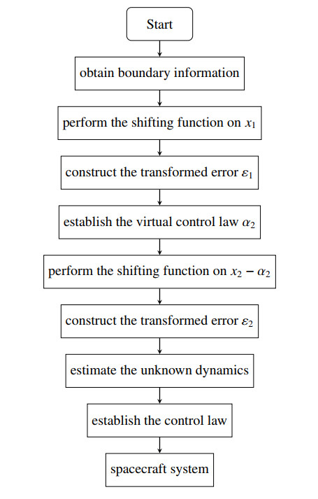
The high-accuracy attitude maneuvering problem for spacecraft systems is investigated. A prescribed performance function and a shifting function are first employed to ensure the predefined-time stability of attitude errors and eliminate the constraints on tracking errors at the incipient stage. Subsequently, a novel predefined-time control scheme is developed by combining prescribed performance control and backstepping control procedures. Radial basis function neural network and minimum learning parameter techniques are introduced to model the function of lumped uncertainty including inertial uncertainties, actuator faults and virtual control law derivatives. According to the rigorous stability analysis, the preset tracking precision can be achieved within a predefined time and the fixed-time boundedness of all closed-loop signals is established. Finally, the efficacy of the propounded control scheme is manifested through numerical simulation results.

Keywords:

Citation: Yuhan Su, Shaoping Shen. Adaptive predefined-time prescribed performance control for spacecraft systems[J]. Mathematical Biosciences and Engineering, 2023, 20(3): 5921-5948. doi: 10.3934/mbe.2023256

Related Papers:

[1]	Ihtisham Ul Haq, Shabir Ahmad, Sayed Saifullah, Kamsing Nonlaopon, Ali Akgül . Analysis of fractal fractional Lorenz type and financial chaotic systems with exponential decay kernels. AIMS Mathematics, 2022, 7(10): 18809-18823. doi: 10.3934/math.20221035
[2]	A. E. Matouk . Chaos and hidden chaos in a 4D dynamical system using the fractal-fractional operators. AIMS Mathematics, 2025, 10(3): 6233-6257. doi: 10.3934/math.2025284
[3]	Nehad Ali Shah, Iftikhar Ahmed, Kanayo K. Asogwa, Azhar Ali Zafar, Wajaree Weera, Ali Akgül . Numerical study of a nonlinear fractional chaotic Chua's circuit. AIMS Mathematics, 2023, 8(1): 1636-1655. doi: 10.3934/math.2023083
[4]	A. M. Alqahtani, Shivani Sharma, Arun Chaudhary, Aditya Sharma . Application of Caputo-Fabrizio derivative in circuit realization. AIMS Mathematics, 2025, 10(2): 2415-2443. doi: 10.3934/math.2025113
[5]	Shabir Ahmad, Aman Ullah, Mohammad Partohaghighi, Sayed Saifullah, Ali Akgül, Fahd Jarad . Oscillatory and complex behaviour of Caputo-Fabrizio fractional order HIV-1 infection model. AIMS Mathematics, 2022, 7(3): 4778-4792. doi: 10.3934/math.2022265
[6]	Rahat Zarin, Abdur Raouf, Amir Khan, Aeshah A. Raezah, Usa Wannasingha Humphries . Computational modeling of financial crime population dynamics under different fractional operators. AIMS Mathematics, 2023, 8(9): 20755-20789. doi: 10.3934/math.20231058
[7]	Khalid K. Ali, K. R. Raslan, Amira Abd-Elall Ibrahim, Mohamed S. Mohamed . On study the fractional Caputo-Fabrizio integro differential equation including the fractional q-integral of the Riemann-Liouville type. AIMS Mathematics, 2023, 8(8): 18206-18222. doi: 10.3934/math.2023925
[8]	Sarkhel Akbar Mahmood, Pshtiwan Othman Mohammed, Dumitru Baleanu, Hassen Aydi, Yasser S. Hamed . Analysing discrete fractional operators with exponential kernel for positivity in lower boundedness. AIMS Mathematics, 2022, 7(6): 10387-10399. doi: 10.3934/math.2022579
[9]	Xiaoyong Xu, Fengying Zhou . Orthonormal Euler wavelets method for time-fractional Cattaneo equation with Caputo-Fabrizio derivative. AIMS Mathematics, 2023, 8(2): 2736-2762. doi: 10.3934/math.2023144
[10]	Rahat Zarin, Amir Khan, Pushpendra Kumar, Usa Wannasingha Humphries . Fractional-order dynamics of Chagas-HIV epidemic model with different fractional operators. AIMS Mathematics, 2022, 7(10): 18897-18924. doi: 10.3934/math.20221041

Abstract

1. Introduction

The complexities of physical phenomena in nature have forced researchers into developing mathematical models that can be used to describe and capture the behavior of these natural occurrences. Traditional calculus may seem to be enough in solving problems that arise from science and engineering. However, many physical phenomena may better be described by fractional calculus because it is a well-suited tool to analyze problems of fractal dimension, with long term "memory" and chaotic behavior ^[1]. Some of the advantages of using fractional calculus over classical calculus are presented by authors in ^[2,3,4,5]. Even though fractional calculus was initially a pure mathematics idea and now regarded as a part of applied mathematics, its application has spread to other fields such as physics ^[3,6], economy ^[4], biology ^{[3,5,7,8,9,10]}, probability^[11], signal processing ^[12], quantitative biology, elasticity, diffusion process, systems identification, viscoelasticity ^[13], transport theory, electrochemistry, rheology, control theory, potential theory, and scattering theory ^[14,15]. Many authors have looked at the theoretical results based on the well-posedness of the fractional differential equations in different forms ^{[16,17,18,19]}. It is clear that for most fractional differential problems, analytical solutions are either impossible to find or are only possible under unrealistic simplifications. As a result, different numerical techniques have been presented by many authors, among which are the variational iteration method, finite difference schemes, Adomain's decomposition, Fourier spectral methods, homotopy analysis methods, A two-step Adams-Bashforth method ^[20], Haar wavelet numerical method ^[21], and many others that have been presented in ^[22].

Another concept that has raised interest in researchers is chaotic systems. Chaotic behavior can be seen in a variety of systems such as fluid dynamics ^[23], population growth, the dynamics of molecular vibration, ecology, electric circuits, the time evolution of the magnetic field of celestial bodies, weather, mechanical devices, and laser ^[24]. Some of the applications of fractional calculus on systems that exhibit chaotic behavior are presented in ^{[25,26,27,28,29,30]}. In this study, we will consider a three-dimensional nonlinear chaotic system called the Lorenz chaotic system ^[31,32,33] introduced by Lorenz ^[34]. This chaotic system opened doors to the development of many other three-dimensional nonlinear chaotic systems such as stretch-twist-fold flow ^[30,35], Chen system ^[36], Rossler system ^[37] and Lui system ^[38].

Recently a new concept of differential and integral operators called fractal-fractional differential and integral operators were introduced by Atangana ^[39], as the convolution of the generalized Mittag-Leffler law, exponential law, and power-law with fractal derivative. These operators consist of two orders, firstly the fractional-order $q$ then the fractal dimension $k$ . The purpose of the new operators is to attract nonlocal problems in nature that also display fractal behavior. The fractal-fractional derivatives find their applications in long-term relation description, macro, and micro-scaled phenomena, discontinuous differential problems, anomalous physical processes ^[40,41,42]. Many authors have looked and these operators and applied them to different fields. Authors such as Qureshi and Atangana ^[43] presented a paper where they used fractal-fractional differentiation to model and analyzed mathematically the dynamics of the transmission of diarrhea that occurred in Ghana between the year $2008$ and $2018$ . A similar study was done by Srivastava, and Saad ^[44]. In their case, they used fractional fractal operators to model the ebola virus. The idea of modeling using fractal fractional derivative was also used by Atangana et al. ^[16] for fractional reaction-diffusion equations. Atangana and Qureshi ^[45] presented a paper where they used the fractional fractal operators to predict chaotic behavior of the Modified Lu Chen attractor, Modified Chua chaotic attractor, Lu Chen attractor, and Chen attractor.

The rest of this paper is arranged in the following way. Under Section 2, we briefly discuss some of the properties and definitions used in this study. The Lorenz Chaotic system under the fractal fractional Caputo Fabrizio derivative is presented in Section 3. In Section 4, we look at the well-posedness of the solution. The numerical scheme is derived in 5. The numerical simulation and graphical results are presented in Section 6. Numerical discussion and error estimate in Sections 7. Lastly, the conclusion is in found Section 8.

2. Preliminaries

In this section, we will give a brief discussion of some important definitions and properties from fractal-fractional calculus that are useful for this paper.

The following definitions are discussed in detail in ^[39].

Definition 2.1. ^[39] Suppose that $u(t)$ is a continuous function and fractal differentiable on an open interval $(a, b)$ with order $k$ then, a $q$ order fractal-fractional derivative of the function $u(t)$ in a Caputo sense with a power-law type kernel is given by:

$\begin{align} &D_{a, t}^{q, k}\big(u(t) \big) = \dfrac{1}{\Gamma(n-q)} \int_{a}^{t}\dfrac{du(s)}{ds^k} (t-s)^{n-q-1}ds, \end{align}$

(2.1)

where $0 < n-1 < q, k \leq n \in \mathbb{N}$ and

$\begin{align*} \dfrac{du(s)}{ds^k} = \lim\limits_{t \rightarrow s}\dfrac{u(x)-u(s)}{t^k-s^k}. \end{align*}$

A generalized version of the above equation is defined as follows:

$\begin{align} &D_{a, t}^{q, k, \theta }\big(u(t) \big) = \dfrac{1}{\Gamma(n-q)} \int_{a}^{t}\dfrac{d^\theta u(s)}{ds^k} (t-s)^{n-q-1}ds, \end{align}$

(2.2)

and

$\begin{align*} \dfrac{d^\theta u(s)}{ds^k} = \lim\limits_{t \rightarrow s}\dfrac{u^\theta(x)-u^\theta(s)}{t^k-s^k}, \end{align*}$

where $\theta \leq 1$ .

Definition 2.2. ^[39] Suppose that $u(t)$ is a continuous function and fractal differentiable on an open interval $(a, b)$ with order $k$ then, a $q$ order fractal-fractional derivative of the function $u(t)$ in a Caputo sense with an exponential decay type kernel is given by:

$\begin{align} &D_{a, t}^{q, k}\big(u(t) \big) = \dfrac{M(q)}{1-q} \int_{a}^{t}\dfrac{du(s)}{ds^k} \exp{\bigg[-\dfrac{q}{1-q}(t-s)\bigg]}ds, \end{align}$

(2.3)

where $0 < q, k \leq n \in \mathbb{N}$ and $M(0) = M(1) = 1.$

A generalized version of the above equation is defined as follows:

$\begin{align} &D_{a, t}^{q, k, \theta}\big(u(t) \big) = \dfrac{M(q)}{1-q} \int_{a}^{t}\dfrac{d^\theta u(s)}{ds^k} \exp{\bigg[-\dfrac{q}{1-q}(t-s)\bigg]}ds, \end{align}$

(2.4)

where $0 < q, k, \theta \leq1$ .

Definition 2.3. ^[39] Suppose that $u(t)$ is a continuous function and fractal differentiable on an open interval $(a, b)$ with order $k$ then, a $q$ order fractal-fractional derivative of the function $u(t)$ in a Caputo sense with the generalized Mittag-Leffler kernel is given by:

$\begin{align} &D_{a, t}^{q, k}\big(u(t) \big) = \dfrac{AB(q)}{1-q} \int_{a}^{t}\dfrac{du(s)}{ds^k} E_q{\bigg(-\dfrac{q}{1-q}(t-s)^q\bigg)}ds, \end{align}$

(2.5)

A generalized version of the above equation is defined as follows:

$\begin{align} &D_{a, t}^{q, k, \theta}\big(u(t) \big) = \dfrac{AB(q)}{1-q} \int_{a}^{t}\dfrac{d^\theta u(s)}{ds^k} E_q{\bigg(-\dfrac{q}{1-q}(t-s)^q\bigg)}ds, \end{align}$

(2.6)

where $0 < \alpha, \beta \leq 1$ and $AB(\alpha) = 1-\alpha+\dfrac{\alpha}{\Gamma(\alpha)}$ .

Definition 2.4. ^[39] Suppose that $u(t)$ is a continuous function and fractal differentiable on an open interval $(a, b)$ with order $k$ then, a $q$ order fractal-fractional derivative of the function $u(t)$ in a Caputo sense with exponential decay kernel is given by:

$\begin{align} &D_{a, t}^{q, k }\big(u(t) \big) = \dfrac{M(q)}{(1-q)} \dfrac{d}{ds^k} \int_{a}^{t}u(s)\exp{\bigg[ -\dfrac{q}{1-q}(t-s)^2\bigg]}ds, \end{align}$

(2.7)

where $0 < q, k\leq n$ and $M(0) = M(1) = 1.$

A generalized version of the above equation is defined as follows:

$\begin{align} &D_{a, t}^{q, k, \theta}\big(u(t) \big) = \dfrac{M(q)}{(1-q)} \dfrac{d^\theta}{ds^k} \int_{a}^{t}u(s)\exp{\bigg[ -\dfrac{q}{1-q}(t-s)^2\bigg]}ds, \end{align}$

(2.8)

where $0 < q, k, \theta\leq 1$ .

Definition 2.5. ^[39] Assuming that $u(t)$ is a continuous function on $(a, b)$ , then a $q$ order fractal-fractional integral of the function $u(t)$ with power law type kernel is given by:

$\begin{align} &J_{a, t}^{q, k}\big(u(t) \big) = \dfrac{k}{\Gamma{(q)}} \int_{a}^{t} (t-s)^{q-1}s^{k-1} u(s)ds. \end{align}$

(2.9)

Definition 2.6. ^[39] Assuming that $u(t)$ is a continuous function on $(a, b)$ , then a $q$ order fractal-fractional integral of the function $u(t)$ with an exponential decaying type kernel is given by:

$\begin{align} &J_{a, t}^{q, k}\big(u(t) \big) = \dfrac{q k}{M(q)} \int_{a}^{t} s^{q-1} u(s)ds + \dfrac{k(1-q)t^{k-1}u(t)}{M(q)}. \end{align}$

(2.10)

Definition 2.7. ^[39] Assuming that $u(t)$ is a continuous function on $(a, b)$ , then a $q$ order fractal-fractional integral of the function $u(t)$ with a generalized Mittag-Leffler type kernel is given by:

$\begin{align} &J_{a, t}^{q, k}\big(u(x) \big) = \dfrac{q k}{AB(q)} \int_{a}^{t} s^{k-1} u(s)(t-s)^{q-1}ds + \dfrac{k(1-q)t^{k-1}u(t)}{AB(q)}. \end{align}$

(2.11)

3. The Lorenz chaotic system under the fractal fractional Caputo-Fabrizio derivative

In this section, we introduce the Lorenz chaotic system under the definition of fractal fractional Caputo-Fabrizio derivative.

Consider the following three dimensional nonlinear chaotic system called the Lorenz chaotic system ^[24,46]

$\begin{align} &x^\prime(t) = \gamma(y-x), \\ &y^\prime (t) = \rho x-y-xz, \\ &z^\prime(t) = xy-\delta z, \end{align}$

(3.1)

where $x = x(t)$ , $y = y(t)$ , and $z = z(t)$ are the dynamical variable of the system and $\gamma$ , $\rho$ , and $\delta$ are the related real constants parameters. Using the definition of the fractal-fractional derivative under the Riemann-Liouville sense with exponential decay kernel for each classical derivative equations in (3.1), we obtain

$\begin{align} &^{RL}D_{0, t}^{q, k}x(t) = \Phi_1(x, y, z, t), \\ &^{RL}D_{0, t}^{q, k}y(t) = \Phi_2(x, y, z, t), \\ &^{RL}D_{0, t}^{q, k}z(t) = \Phi_3(x, y, z, t), \end{align}$

(3.2)

where $\Phi_1(x, y, z, t) = \gamma(y-x)$ , $\Phi_2(x, y, z, t) = \rho x-y-xz,$ and $\Phi_3(x, y, z, t) = xy-\delta z$ . The above system of equations can be written as follows

$\begin{align} &^{RL}D_{0, t}^{q, k}x(t) = \dfrac{M(q)}{1-q} \dfrac{d}{dt^k}\int_{0}^{t}\exp{\bigg(-\dfrac{q}{1-q}(t-s) \bigg)}\Phi_1(x, y, z, s)ds, \\ &^{RL}D_{0, t}^{q, k}y(t) = \dfrac{M(q)}{1-q} \dfrac{d}{dt^k}\int_{0}^{t}\exp{\bigg(-\dfrac{q}{1-q}(t-s) \bigg)}\Phi_2(x, y, z, s)ds, \\ &^{RL}D_{0, t}^{q, k}z(t) = \dfrac{M(q)}{1-q} \dfrac{d}{dt^k}\int_{0}^{t}\exp{\bigg(-\dfrac{q}{1-q}(t-s) \bigg)}\Phi_3(x, y, z, s)ds. \end{align}$

(3.3)

Since the fractional integral is differentiable. We can rewrite the Eq (3.3) as

$\begin{align} &^{RL}D_{0, t}^{q, k}x(t) = \dfrac{M(q)}{1-q} \dfrac{d}{dt}\int_{0}^{t}\exp{\bigg(-\dfrac{q}{1-q}(t-s) \bigg)}\Phi_1(x, y, z, s)ds\dfrac{1}{kt^{k-1}}, \\ &^{RL}D_{0, t}^{q, k}y(t) = \dfrac{M(q)}{1-q} \dfrac{d}{dt}\int_{0}^{t}\exp{\bigg(-\dfrac{q}{1-q}(t-s) \bigg)}\Phi_2(x, y, z, s)ds\dfrac{1}{kt^{k-1}}, \\ &^{RL}D_{0, t}^{q, k}z(t) = \dfrac{M(q)}{1-q} \dfrac{d}{dt}\int_{0}^{t}\exp{\bigg(-\dfrac{q}{1-q}(t-s) \bigg)}\Phi_3(x, y, z, s)ds\dfrac{1}{kt^{k-1}}. \end{align}$

(3.4)

Therefore, system (3.4) can be expressed as follows

$\begin{align} &^{RL}D_{0, t}^{q, k}x(t) = kt^{k-1}\Phi_1(x, y, z, t), \\ &^{RL}D_{0, t}^{q, k}y(t) = kt^{k-1}\Phi_2(x, y, z, t), \\ &^{RL}D_{0, t}^{q, k}z(t) = kt^{k-1}\Phi_3(x, y, z, t). \end{align}$

(3.5)

We now replace the Riemann-Liouville derivative with the Caputo-Fabrizio derivative to make use of the integer-order initial conditions. Thus from system (3.5) we get

$\begin{align} &^{CF}D_{0, t}^{q, k}x(t) = kt^{k-1}\Phi_1(x, y, z, t), \\ &^{CF}D_{0, t}^{q, k}y(t) = kt^{k-1}\Phi_2(x, y, z, t), \\ &^{CF}D_{0, t}^{q, k}z(t) = kt^{k-1}\Phi_3(x, y, z, t). \end{align}$

(3.6)

In this study, we will investigate the above system of equations.

4. The well-posedness of the fractal fractional Caputo-Frabrizio derivative of the Lorenz system

In this section, we use the Pichard Lindelof method ^[46,47,48] to show the existence and uniqueness of the solution of the following nonlinear system of equations

(4.1)

subjected to the following initial conditions

$\begin{align} &x(0) = x_0, \\ &y(0) = y_0, \\ &z(0) = z_0. \end{align}$

To show the existence and uniqueness of the solution we define the following operators.

$\begin{align} &f_1(t, x) = \gamma(y-x), \\ &f_2 (t, y) = \rho x-y-xz, \\ &f_3(t, z) = xy-\delta z, \end{align}$

(4.2)

Now, let

$\begin{align} &C_{a, b_1} = A_1 \times B_1, \\ &C_{a, b_2} = A_2 \times B_2, \\ &C_{a, b_3} = A_3 \times B_3, \end{align}$

(4.3)

where

$\begin{align} &A_1 = A_2 = A_3 = [t_0-a, t_0+a] , \\ &B_1 = [x_0-b_1, x_0+b_1] , \\ &B_2 = [y_0-b_2, y_0+b_2] , \\ &B_3 = [z_0-b_3, z_0+b_3] , \end{align}$

(4.4)

We now want to show that $f_1, f_2$ and $f_3$ satisfy the Lipschipitz conditions with respect to $x, y, z$ respectively. This means that for any two given functions $\psi_1, \psi_2 \in C(A_1, B_1, B_2, B_3)$ there exists a positive constant $k$ such that

$\begin{align*} \big\|f(t, \psi_1)-f(t, \psi_2)\big\| \leq k \big\|\psi_1-\psi_2\big\| . \end{align*}$

For $f_1$ we have

$\begin{align} \big\|f_1(t, \psi_1)-f_1(t, \psi_2)\big\|& = \big\|(\gamma y(t)-\gamma\psi_1))-(\gamma y(t)-\gamma \psi_2)\big\| \\ & = \big\|-\gamma \psi_1+ \gamma \psi_2\big\| \\ & = \big\|-\gamma (\psi_1-\psi_2)\big\| \\ &\leq |\gamma|\big\|\psi_1-\psi_2\big\|. \end{align}$

(4.5)

Hence, $f_1$ is satisfies the Lipschipitz conditions. For $f_2$ we have

$\begin{align} \big\|f_2(t, \psi_1)-f_2(t, \psi_2)\big\|& = \big\|(\rho x(t)-\psi_1-x(t)z(t))-( \rho x(t)-\psi_2-x(t)z(t))\big\| \\ & = \big\|-\psi_1+\psi_2\big\| \\ & = \big\|-(\psi_1-\psi_2\big)\| \\ &\leq \big\|\psi_1-\psi_2\big\|. \end{align}$

(4.6)

Thus, $f_2$ is satisfies the Lipschipitz conditions. For $f_3$ we have

$\begin{align} \big\|f_3(t, \psi_1)-f_3(t, \psi_2)\big\|& = \big\|(x(t)y(t)-\delta \psi_1)-(x(t)y(t)-\delta \psi_2))\big\| \\ & = \big\|-\delta \psi_1+\delta \psi_2\big\| \\ & = \big\|-\delta (\psi_1-\psi_2\big)\| \\ &\leq|\delta| \big\|\psi_1-\psi_2\big\|. \end{align}$

(4.7)

Therefore, $f_3$ satisfies the Lipschipitz conditions.

Now, let

$\begin{align} &M_1 = \sup\limits_{C_{a, b_1}} \, |f_1(t, x)|, \\ &M_2 = \sup\limits_{C_{a, b_2}} \, |f_2(t, y)|, \\ &M_3 = \sup\limits_{C_{a, b_3}} \, |f_3(t, z)|, \end{align}$

(4.8)

We now continue to apply the Banach fixed point theorem using the metric on spaces of continuous functions $C(A_1, B_1, B_2, B_3)$ induced by the norm

$\begin{align} \big\|f(t)\big\|_\infty & = \sup\limits_{t \in [t_0-a, t_0+a]} \, |f(t)|. \end{align}$

(4.9)

We now define the next operator between the two functional spaces of continuous functions, Picard's operator, as follows

$\begin{align} D:C(A_1, B_1, B_2, B_3)\rightarrow C(A_1, B_1, B_2, B_3). \end{align}$

(4.10)

Defined as follows

$\begin{align} DX(t) = X_0(t)+ \frac{k t^{k-1}(1-q)}{M(q)}F(t, X(t))+\frac{q k}{M(q)}\int_{0}^{t} \Lambda^{\tau-1}F(\Lambda, X(\Lambda)) d \Lambda \end{align}$

(4.11)

Where the matrix $X$ is given as

$\begin{align*} X(t) = \begin{bmatrix} x(t) \\ y(t) \\ z(t) \end{bmatrix}\\ \end{align*}$

$\begin{align*} X_0(t) = \begin{bmatrix} x_0 \\ y_0 \\ z_0 \end{bmatrix}\\ \end{align*}$

and

$\begin{align*} F(t, X(t)) = \begin{bmatrix} f_1(t, x) \\ f_2(t, y)\\ f_3(t, z) \end{bmatrix}\\ \end{align*}$

From (4.5)–(4.7) we can conclude that $F(t, X(t))$ satisfies Lipschipitz conditions with respect to the system state variable $X(t)$ . Now, we must show that this operator maps a complete nonempty space into itself. We first show that, given a certain restriction on $a$ , $D$ takes values in $B_1, B_2, B_3$ in the space of continuous functions with uniform norm. To obtain good results, we assume that the problem under consideration satisfies

$\begin{align*} \|X(t)\|_{\infty} = \max \{b_1, b_2, b_3\} = b \end{align*}$

implies

$\begin{align} \big\|DX(t)-X_0(t)\big\|& = \bigg\|\frac{k t^{k-1}(1-q)}{M(q)}F(t, X(t))+\frac{q k}{M(q)}\int_{0}^{t} \Lambda^{k-1}F(\Lambda, X(\Lambda)) d \Lambda \bigg\| \\ &\leq \frac{k t^{k-1}(1-q)}{M(q)}\big\|F(t, X(t))\big\|+\frac{q k}{M(q)}\int_{0}^{t} \Lambda^{k-1}\big\|F(\Lambda, X(\Lambda)) d \Lambda \big\| \\ &\leq \frac{k t^{k-1}(1-q)}{M(q)}M+\frac{q k}{M(q)}.\frac{Ma^k}{k} \\ &\leq Ma \\ &\leq b, \\ \end{align}$

(4.12)

where $b = \max\{b_1, b_2, b_3\}$ and $M = \max\{M_1, M_2, M_3\}$ . The last step is true if we impose the requirement $a < \frac{b}{M}$ .

Using the maximum's metric

$\begin{align} \big\|DX_1-DX_2\big\|_\infty & = \sup\limits_{t \in [t_0-a, t_0+a]} \, |X_1-X_2|. \end{align}$

(4.13)

We want to show that the operator is a contraction mapping. So, we have

$\begin{align} \big\|DX(t)-X_0(t)\big\|& = \bigg\|\frac{ t^{k-1}(1-q)}{M(q)}\big[F(t, X_1(t))-F(t, X_2(t))\big] \\ &+\frac{q k}{M(q)}\int_{0}^{t} \Lambda^{k-1}\big[F(\Lambda, X_1(\Lambda))-F(\Lambda, X_2(\Lambda))\big] d \Lambda \bigg\| \\ &\leq \frac{k t^{k-1}(1-q)}{M(q)}\big\|F(t, X_1(t))-F(t, X_2(t))\big\| \\ &+\frac{q k}{M(q)}\int_{0}^{t} \lambda^{k-1}\big\|F(\Lambda, X_1(\Lambda))-F(\Lambda, X_2(\Lambda))\big\| d \Lambda \\ &\leq \frac{k t^{k-1}(1-q)}{M(q)}p\big\|X_1(t)-X_2(t)\big\|+\frac{q k}{M(q)}\int_{0}^{t} \Lambda^{k-1}\big\|F(\Lambda, X_1(\Lambda))-F(\Lambda, X_2(\Lambda))\big\| d \Lambda \\ \text{F is Lipschitz continuous} \\ &\leq \frac{k t^{k-1}(1-q)}{M(q)}p\big\|X_1(t)-X_2(t)\big\|+\frac{qa^k p}{M(q)}\big\|X_1(t)-X_2(t)\big\| \\ & = \bigg( \frac{pkt^{k-1}(1-q)}{M(q)} +\frac{q a^k p}{M(q)} \bigg)\big\|X_1(t)-X_2(t)\big\| \\ &\leq ap\big\|X_1(t)-X_2(t)\big\| \end{align}$

(4.14)

with $p < 1$ . Since $F$ is Lipschitz continuous, we have that the operator $D$ is a contraction for $a rp < 1$ . Hence, this shows that the system under consideration has a unique set of solution.

5. Numerical scheme

In this section, we present the numerical scheme for the Caputo Fabrizio fractal fractional derivative of the Lorenz chaotic system. The chaotic model (3.1) can be converted to

(5.1)

Where

$\begin{align*} &\Phi_1(x, y, z, t) = \gamma(y-x), \\ &\Phi_2(x, y, z, t) = \rho x-y-xz, \\ &\Phi_2(x, y, z, t) = xy-\delta z. \end{align*}$

When we apply the Caputo-Fabrizio integral to (5.1), we get

$\begin{align} &x(t)-x(0) = \frac{k t^{k-1}(1-q)}{M(q)}\Phi_1(x, y, z, t)+\frac{q k}{M(q)}\int_{0}^{t} \Lambda^{k-1}\Phi_1(x, y, z, \Lambda) d \Lambda, \\ &y(t)-y(0) = \frac{k t^{k-1}(1-q)}{M(q)}\Phi_2(x, y, z, t)+\frac{q k}{M(q)}\int_{0}^{t} \Lambda^{k-1}\Phi_2(x, y, z, \Lambda) d \Lambda , \\ &z(t)-z(0) = \frac{k t^{k-1}(1-q)}{M(q)}\Phi_3(x, y, z, t)+\frac{q k}{M(q)}\int_{0}^{t} \Lambda^{k-1}\Phi_3(x, y, z, \Lambda) d \Lambda. \end{align}$

(5.2)

For a positive integer $n$ , the solution of the system of Eq (5.1) at $t = t_{n+1}$ becomes,

$\begin{align} &x(t_{n+1})-x(0) = \frac{k t^{k-1}_{n}(1-q)}{M(q)}\Phi_1(x(t_{n}), y(t_{n}), z(t_{n}), t_n)+\frac{q k}{M(q)}\int_{0}^{t_{n+1}} \Lambda^{k-1}\Phi_1(x, y, z, \Lambda) d \Lambda, \\ &y(t_{n+1})-y(0) = \frac{k t^{k-1}_{n}(1-q)}{M(q)}\Phi_2(x(t_{n}), y(t_{n}), z(t_{n}), t_n)+\frac{q k}{M(q)}\int_{0}^{t_{n+1}} \Lambda^{k-1}\Phi_2(x, y, z, \Lambda) d \Lambda , \\ &z(t_{n+1})-z(0) = \frac{k t^{k-1}_{n}(1-q)}{M(q)}\Phi_3(x(t_{n}), y(t_{n}), z(t_{n}), t_n)+\frac{q k}{M(q)}\int_{0}^{t_{n+1}} \Lambda^{k-1}\Phi_3(x, y, z, \Lambda) d \Lambda. \end{align}$

(5.3)

and at $t = t_{n}$ , we obtain

$\begin{align} &x(t_{n})-x(0) = \frac{k t^{k-1}_{n-1}(1-q)}{M(q)}\Phi_1(x(t_{n-1}), y(t_{n-1}), z(t_{n-1}), t_{n-1})+\frac{q k}{M(q)}\int_{0}^{t_{n}} \Lambda^{k-1}\Phi_1(x, y, z, \Lambda) d \Lambda, \\ &y(t_{n})-y(0) = \frac{k t^{k-1}_{n-1}(1-q)}{M(q)}\Phi_2(x(t_{n-1}), y(t_{n-1}), z(t_{n-1}), t_{n-1})+\frac{q k}{M(q)}\int_{0}^{t_{n}} \Lambda^{k-1}\Phi_2(x, y, z, \Lambda) d \Lambda , \\ &z(t_{n})-z(0) = \frac{k t^{k-1}_{n-1}(1-q)}{M(q)}\Phi_3(x(t_{n-1}), y(t_{n-1}), z(t_{n-1}), t_{n-1})+\frac{q k}{M(q)}\int_{0}^{t_{n}} \Lambda^{k-1}\Phi_3(x, y, z, \Lambda) d \Lambda. \end{align}$

(5.4)

Taking the difference between (5.4) and (5.3), we get

$\begin{align} &x(t_{n+1})-x(t_{n}) = \frac{k t^{k-1}_{n}(1-q)}{M(q)}\Phi_1(x(t_{n}), y(t_{n}), z(t_{n}), t_{n}) \\ & \qquad \qquad \qquad \quad- \frac{k t^{k-1}_{n-1}(1-q)}{M(q)}\Phi_1(x(t_{n-1}), y(t_{n-1}), z(t_{n-1}), t_{n-1}) \\ & \qquad \qquad \qquad \quad +\frac{q k}{M(q)}\int_{t_{n}}^{t_{n+1}} \Lambda^{k-1}\Phi_1(x, y, z, \Lambda) d \Lambda, \\ &y(t_{n+1})-y(t_{n}) = \frac{k t^{k-1}_{n}(1-q)}{M(q)}\Phi_2(x(t_{n}), y(t_{n}), z(t_{n}), t_{n}) \\ & \qquad \qquad \qquad \quad- \frac{k t^{k-1}_{n-1}(1-q)}{M(q)}\Phi_2(x(t_{n-1}), y(t_{n-1}), z(t_{n-1}), t_{n-1}) \\ & \qquad \qquad \qquad \quad +\frac{q k}{M(q)}\int_{t_{n}}^{t_{n+1}} \Lambda^{k-1}\Phi_1(x, y, z, \Lambda) d \Lambda, \\ &z(t_{n+1})-z(t_{n}) = \frac{k t^{k-1}_{n}(1-q)}{M(q)}\Phi_3(x(t_{n}), y(t_{n}), z(t_{n}), t_{n}) \\ & \qquad \qquad \qquad \quad -\frac{k t^{k-1}_{n-1}(1-q)}{M(q)}\Phi_3(x(t_{n-1}), y(t_{n-1}), z(t_{n-1}), t_{n-1}) \\ & \qquad \qquad \qquad \quad +\frac{q k}{M(q)}\int_{t_{n}}^{t_{n+1}} \Lambda^{k-1}\Phi_3(x, y, z, \Lambda) d \Lambda. \end{align}$

(5.5)

We now approximate the functions $\Lambda^{k-1}\Phi_1(x, y, z, \Lambda)$ , $\Lambda^{k-1}\Phi_2(x, y, z, \Lambda)$ and $\Lambda^{k-1}\Phi_3(x, y, z, \Lambda)$ on the finite interval $[t_n, t_{n+1}]$ using the piece-wise Lagrangian interpolation such as

$\begin{align} &Q_1(\Lambda) = \dfrac{\Lambda-t_{n-1}}{t_n-t_{n-1}}t_n^{k-1}\Phi_1(x(t_{n}), y(t_{n}), z(t_{n}), t_{n})-\dfrac{\Lambda-t_{n}}{t_n-t_{n-1}}t_{n-1}^{k-1}\Phi_1(x(t_{n-1}), y(t_{n-1}), z(t_{n-1}), t_{n-1}), \\ &Q_2(\Lambda) = \dfrac{\Lambda-t_{n-1}}{t_n-t_{n-1}}t_n^{k-1}\Phi_2(x(t_{n}), y(t_{n}), z(t_{n}), t_{n})-\dfrac{\Lambda-t_{n}}{t_n-t_{n-1}}t_{n-1}^{k-1}\Phi_2(x(t_{n-1}), y(t_{n-1}), z(t_{n-1}), t_{n-1}), \\ &Q_3(\Lambda) = \dfrac{\Lambda-t_{n-1}}{t_n-t_{n-1}}t_n^{k-1}\Phi_3(x(t_{n}), y(t_{n}), z(t_{n}), t_{n})-\dfrac{\Lambda-t_{n}}{t_n-t_{n-1}}t_{n-1}^{k-1}\Phi_3(x(t_{n-1}), y(t_{n-1}), z(t_{n-1}), t_{n-1}). \end{align}$

(5.6)

Substituting (5.6) into (5.5) and integrating, we obtain

$\begin{align} &x(t_{n+1})-x(t_{n}) = kt_n^{k-1}\bigg( \frac{3q\triangle t}{2M(q)} +\dfrac{(1-q)}{M(q)}\bigg)\Phi_1(x(t_{n}), y(t_{n}), z(t_{n}), t_{n}) \\ & \qquad \qquad \qquad \quad-kt_{n-1}^{k-1}\bigg( \frac{q\triangle t}{2M(q)} +\dfrac{(1-q)}{M(q)}\bigg)\Phi_1(x(t_{n-1}), y(t_{n-1}), z(t_{n-1}), t_{n-1}), \\ &y(t_{n+1})-y(t_{n}) = kt_n^{k-1}\bigg( \frac{3q\triangle t}{2M(q)} +\dfrac{(1-q)}{M(q)}\bigg)\Phi_2(x(t_{n}), y(t_{n}), z(t_{n}), t_{n}) \\ & \qquad \qquad \qquad \quad-kt_{n-1}^{k-1}\bigg( \frac{q\triangle t}{2M(q)} +\dfrac{(1-q)}{M(q)}\bigg)\Phi_2(x(t_{n-1}), y(t_{n-1}), z(t_{n-1}), t_{n-1}), \\ &z(t_{n+1})-z(t_{n}) = kt_n^{k-1}\bigg( \frac{3q\triangle t}{2M(q)} +\dfrac{(1-q)}{M(q)}\bigg)\Phi_3(x(t_{n}), y(t_{n}), z(t_{n}), t_{n}) \\ & \qquad \qquad \qquad \quad-kt_{n-1}^{k-1}\bigg( \frac{q\triangle t}{2M(q)} +\dfrac{(1-q)}{M(q)}\bigg)\Phi_3(x(t_{n-1}), y(t_{n-1}), z(t_{n-1}), t_{n-1}), \end{align}$

(5.7)

Therefore, we have completed the derivation of the numerical scheme used in this study.

6. Numerical simulation

In the previous section, we presented a numerical scheme under the Caputo-Fabrizio fractal-fractional derivative operator. In this section, we aim to use the numerical scheme presented to approximate the graphical solution for the Lorenz chaotic systems under the Caputo-Fabrizio fractal-fractional derivative operator for different values of the fractional dimension $q$ and the fractal dimension $k$ . We now look at the following examples:

Example 1. Consider the following system of equations

(6.1)

where $\Phi_1(x, y, z, t) = \gamma(y-x)$ , $\Phi_2(x, y, z, t) = \rho x-y-xz,$ and $\Phi_2(x, y, z, t) = xy-\delta z$ . With parameter values $\gamma = 10$ , $\rho = 28$ and $\delta = \dfrac{8}{3}$ . In this example we solve the system (6.1) using the initial conditions $x(0) = y(0) = z(0) = -1$ . The graphical numerical simulations for different values of $q$ and $k$ for this example are presented in Figures 1–4.

Figure 1. The dynamical behavior of the Lorenz chaotic system (6.1), using the Caputo-Fabrizio fractal-fractional derivative operator for different values of

$k$ and

$q$ .

DownLoad: Full-Size Img PowerPoint

Figure 2. The dynamical behavior of the Lorenz chaotic system (6.1), using the Caputo-Fabrizio fractal-fractional derivative operator for different values of

$k$ and

$q$ .

DownLoad: Full-Size Img PowerPoint

Figure 3. The dynamical behavior of the Lorenz chaotic system (6.1), using the Caputo-Fabrizio fractal-fractional derivative operator for different values of

$k$ and

$q$ .

DownLoad: Full-Size Img PowerPoint

Figure 4. The dynamical behavior of the Lorenz chaotic system (6.1), using the Caputo-Fabrizio fractal-fractional derivative operator for different values of

$k$ and

$q$ .

DownLoad: Full-Size Img PowerPoint

Example 2. For the the second example, we consider the system of equation in example 1 with different initial conditions. Consider the following system of equations

(6.2)

In this example, we solve the system (6.2) using the initial conditions $x(0) = 0$ , $y(0) = 2$ and $z(0) = 20$ . The graphical numerical simulations for different values of $q$ and $k$ for this example are presented in Figures 5–8.

Figure 5. The dynamical behavior of the Lorenz chaotic system (6.1), using the Caputo-Fabrizio fractal-fractional derivative operator for different values of

$k$ and

$q$ .

DownLoad: Full-Size Img PowerPoint

Figure 6. The dynamical behavior of the Lorenz chaotic system (6.1), using the Caputo-Fabrizio fractal-fractional derivative operator for different values of

$k$ and

$q$ .

DownLoad: Full-Size Img PowerPoint

Figure 7. The dynamical behavior of the Lorenz chaotic system (6.1), using the Caputo-Fabrizio fractal-fractional derivative operator for different values of

$k$ and

$q$ .

DownLoad: Full-Size Img PowerPoint

Figure 8. The dynamical behavior of the Lorenz chaotic system (6.1), using the Caputo-Fabrizio fractal-fractional derivative operator for different values of

$k$ and

$q$ .

DownLoad: Full-Size Img PowerPoint

7. Discussion

In Example $1$ and $2$ , we modeled the Lorenz chaotic system with initial conditions $x(0) = y(0) = z(0) = -1$ and $x(0) = 0, \, \, y(0) = 2$ and $z(0) = 20$ respectively, using the Caputo-Fabrizio fractal-fractional derivative operator. We then solved the obtained nonlinear systems of equations using a numerical scheme for different fractal dimensions $k$ and fractional order $q$ . – represent the graphical simulation, for example, $1$ , and – represent the graphical simulation, for example $2$ . In both examples, we noticed that the fractal power $k = 1$ and the fractional power $q = 1$ recover the classical two-step Adams-Bashforth method and the classical differential and integral operators. and represents the graphical solutions for the case where $k = 1$ and $q = 1$ for example $1$ and example $2$ , respectively. While solving the systems of equations, we noticed that for some values of $k$ and $q$ the solution blows up.

For both examples, we noticed that if we keep $q = 1$ and vary the value of $k$ we can obtain graphical solutions for as far as $k = 0.10$ , see and but if we make $k = 1$ and vary the value of $q$ the solution of the nonlinear system of equation blows up for some values of $q$ . Keeping one variable constant and varying the others, we noticed that for the following values some values of $k$ and $q$ the solutions blow up, see Figure 2(d), 3(b), 3(d), 3(f), , – and for example $2$ , see Figure 6(c), 6(g), 7(b), 7(e), 7(g), 8(a), 8(c) and 8(f)–(h).

Taking into consideration that the chaotic systems are sensitive to initial conditions. Comparing the values for which the solution blows up between the two examples might give us an idea of the factors contributing to the blowing up of the solution. The following table shows a comparison of the values for which the solution blows up.

From , we can see that the solution for Example $1$ for some values of $k$ and $q$ blows up faster than those in Example $2$ . This means that the choice of the initial conditions of the nonlinear system of equations also contributes to when the solution blows up for the nonlinear system under investigation.

Table 1. Comparison of the values for which the solution blows up for both examples.

Constant values	Example 1	Example 2
$k=1$	$0 < q\leq 0.95$	$0 < q\leq 0.94$
$q=0.99$	$0 < k \leq 0.81$	$0 < k \leq 0.78$
$k=0.99$	$0 < q\leq 0.95$	$0 < q\leq 0.94$
$q=0.98$	$0 < k\leq 0.89$	$0 < k\leq 0.86$
$k=0.98$	$0 < q\leq 0.96$	$0 < q\leq 0.94$
$q=0.97$	$0 < k\leq 0.94$	$0 < k\leq 0.91$
$k=0.97$	$0 < q\leq 0.96$	$0 < q\leq 0.95$
$q=0.96$	$0 < k\leq 0.96$	$0 < k\leq 0.94$
$k=0.96$	$0 < q\leq 0.96$	$0 < q\leq 0.95$
$0 < k\leq 1$	$0 < q\leq 0.94$	$0 < q\leq 0.94$
$0 < q\leq 0.96$	$0 < k\leq 0.95$	$0 < k\leq 0.94$

| Show Table

DownLoad: CSV

7.1. Error estimate

In this section, we use numerical results obtained from the numerical scheme to estimate the rate of convergence using the following

$\begin{align*} p = \frac{\log \bigg|\frac{u^{\frac{h}{2}-u^{h}}}{u^{\frac{h}{4}}-u^\frac{h}{2}}\bigg|}{\log2} \end{align*}$

where $u^h = \{x^h(t), y^h(t), z^h(t)\}$ , $u^{\frac{h}{2}} = \{x^\frac{h}{2}(t), y^\frac{h}{2}(t), z^\frac{h}{2}(t)\}$ and $u^{\frac{h}{4}} = \{x^\frac{h}{4}(t), y^\frac{h}{4}(t), z^\frac{h}{4}(t)\}$ are the approximate solutions to $u(x) = \{x(t), y(t), z(t)\}$ for the step size $h$ , $\frac{h}{2}$ and $\frac{h}{4}$ respectively.

The results in Tables 2–7 depict order one and two rate of convergence. However, this approach might not be entirely reliable because we deal with chaotic systems that are extremely sensitive to initial conditions. Some other methods are proposed in ^[49,50].

Table 2. The rate of convergence for different values of

$h$ using example 1.

$h$	$x(t)$	$p$
$\frac{1}{100}$	$-$ 1.230587514160928	1.904959580936555
$\frac{1}{200}$	$-$ 1.061110242113278	1.940190794821020
$\frac{1}{400}$	$-$ 1.015855771334397	1.961017182073904
$\frac{1}{800}$	$-$ 1.004063271904520	1.972167801697337
$\frac{1}{1600}$	$-$ 1.001034400255673	1.977926785981624
$\frac{1}{3200}$	$-$ 1.000262432420641	1.980853052009642
$\frac{1}{6400}$	$-$ 1.000066464983257
$\frac{1}{12800}$	$-$ 1.000016818587168

| Show Table

DownLoad: CSV

Table 3. The rate of convergence for different values of

$h$ using example 1.

$h$	$y(t)$	$p$
$\frac{1}{100}$	$-$ 2.326508213491328	1.067858535219673
$\frac{1}{200}$	$-$ 1.647800735475855	1.006794709692697
$\frac{1}{400}$	$-$ 1.324039249963567	0.992944397031469
$\frac{1}{800}$	$-$ 1.162919129852769	0.990829292631269
$\frac{1}{1600}$	$-$ 1.081964120101717	0.991036225398347
$\frac{1}{3200}$	$-$ 1.041228494373794	0.991461358994093
$\frac{1}{6400}$	$-$ 1.020733737952112	0.991752429070755
$\frac{1}{12800}$	$-$ 1.010425530442698	0.991914116840363
$\frac{1}{25600}$	$-$ 1.005241877425116	0.991995057252036
$\frac{1}{51200}$	$-$ 1.002635483703504
$\frac{1}{102400}$	$-$ 1.001325035822124

| Show Table

DownLoad: CSV

Table 4. The rate of convergence for different values of

$h$ using example 1.

$h$	$z(t)$	$p$
$\frac{1}{100}$	$-$ 0.810858602235998	1.134148250045712
$\frac{1}{200}$	$-$ 0.910831556058634	1.051723457397754
$\frac{1}{400}$	$-$ 0.956379615764291	1.020129659296684
$\frac{1}{800}$	$-$ 0.978351614908976	1.005880122139417
$\frac{1}{1600}$	$-$ 0.989185393271114	0.998981951425179
$\frac{1}{3200}$	$-$ 0.994580249280774	0.995555981083686
$\frac{1}{6400}$	$-$ 0.997279581417658
$\frac{1}{12800}$	$-$ 0.998633411352176

| Show Table

DownLoad: CSV

Table 5. The rate of convergence for different values of

$h$ using example 2.

$h$	$x(t)$	$p$
$\frac{1}{100}$	0.751972948680281	0.785531902054452
$\frac{1}{200}$	0.415109454355213	0.879128933122776
$\frac{1}{400}$	0.219682130799205	0.933763944099137
$\frac{1}{800}$	0.113429154201297	0.962477934907692
$\frac{1}{1600}$	0.057806699720829	0.977150215826183
$\frac{1}{3200}$	0.029262661073358	0.984573990764699
$\frac{1}{6400}$	0.014762798186914
$\frac{1}{12800}$	0.007434930967961

| Show Table

DownLoad: CSV

Table 6. The rate of convergence for different values of

$h$ using example 2.

$h$	$y(t)$	$p$
$\frac{1}{100}$	2.063882999678037	3.578639814091108
$\frac{1}{200}$	1.992390832959806	0.463370460207230
$\frac{1}{400}$	1.986406985255091	0.118777817473332
$\frac{1}{800}$	1.990747009184933	0.699165428640857
$\frac{1}{1600}$	1.994744030260617	0.865555010973675
$\frac{1}{3200}$	1.997205909082042	0.932675206008964
$\frac{1}{6400}$	1.998557074903865
$\frac{1}{12800}$	1.999264931751799

| Show Table

DownLoad: CSV

Table 7. The rate of convergence for different values of

$h$ using example 2.

$h$	$z(t)$	$p$
$\frac{1}{100}$	17.710724336596417	0.919794628750672
$\frac{1}{200}$	18.810610778750505	0.955734196405311
$\frac{1}{400}$	19.391993440099736	0.973775158693165
$\frac{1}{800}$	19.691742213503858	0.982881681370900
$\frac{1}{1600}$	19.844365880125473	0.987471151984859
$\frac{1}{3200}$	19.921588585883410	0.989778019827995
$\frac{1}{6400}$	19.960536712925116
$\frac{1}{12800}$	19.980149246718597

| Show Table

DownLoad: CSV

8. Conclusions

In this study, we used the newly proposed Caputo Fabrizio fractal fractional operator with different fractal dimension $k$ and fractional order $q$ , to capture and analyze the dynamical behavior of the Lorenz chaotic system. We present the numerical scheme used to solve the system of nonlinear equations and obtained graphical numerical simulations for different values of $q$ and $k$ . We noticed that for the fractal dimension $k = 1$ and fractional order $q = 1$ we obtain a two-step Adams Bashforth method and the classical differential and integral operators. We also noticed that for some values of $q$ and $k$ the solutions blow up. Taking into consideration that the chaotic systems are sensitive to initial conditions we compared two examples of the same nonlinear system of equations with different initial conditions, we noticed that the choice of the initial conditions also affect when some solutions blow up. For future work, we want to find out what other factors contribute to the blowing up of the solutions for some values of $q$ and $k$ .

Acknowledgments

The authors are grateful to the referees for providing valuable comments and helpful suggestions on the paper.

Conflict of interest

The authors declare no conflict of interest.

References

[1]	K. Xia, Y. Eun, T. Lee, S. Y. Park, Integrated adaptive control for spacecraft attitude and orbit tracking using disturbance observer, Int. J. Aeronaut. Space Sci., 22 (2021), 936–947. https://doi.org/10.1007/s42405-021-00359-x doi: 10.1007/s42405-021-00359-x
[2]	X. Chen, L. Zhao, Observer-based finite-time attitude containment control of multiple spacecraft systems, IEEE Trans. Circuits Syst. II Express Briefs, 68 (2020), 1273–1277. https://doi.org/10.1109/TCSII.2020.3024941 doi: 10.1109/TCSII.2020.3024941
[3]	R. Nadafi, M. Kabganian, Robust nonlinear attitude tracking control of an underactuated spacecraft under saturation and time-varying uncertainties, Eur. J. Control, 63 (2022), 133–142. https://doi.org/10.1016/j.ejcon.2021.09.003 doi: 10.1016/j.ejcon.2021.09.003
[4]	Q. Hu, B. Li, M. I. Friswell, Observer-based fault diagnosis incorporating online control allocation for spacecraft attitude stabilization under actuator failures, J. Astronaut. Sci., 60 (2013), 211–236. https://doi.org/10.1007/s40295-014-0021-1 doi: 10.1007/s40295-014-0021-1
[5]	M. Z. Dai, B. Xiao, C. Zhang, J. Wu, Event-triggered policy to spacecraft attitude stabilization with actuator output nonlinearities, IEEE Trans. Circuits Syst. II Express Briefs, 68 (2021), 2855–2859. https://doi.org/10.1109/TCSII.2021.3056761 doi: 10.1109/TCSII.2021.3056761
[6]	Q. Liu, M. Liu, G. Duan, Adaptive fuzzy backstepping control for attitude stabilization of flexible spacecraft with signal quantization and actuator faults, Sci. China Inf. Sci., 64 (2021), 1–16. https://doi.org/10.1007/s11432-020-2949-5 doi: 10.1007/s11432-020-2949-5
[7]	S. P. Bhat, D. S. Bernstein, Finite-time stability of continuous autonomous systems, SIAM J. Control Optim., 38 (2000), 751–766. https://doi.org/10.1137/S0363012997321358 doi: 10.1137/S0363012997321358
[8]	Z. Xiong, X. Li, M. Ye, Q. Zhang, Finite-time stability and optimal control of an impulsive stochastic reaction-diffusion vegetation-water system driven by lévy process with time-varying delay, Math. Biosci. Eng., 18 (2021), 8462–8498. https://doi.org/10.3934/mbe.2021419 doi: 10.3934/mbe.2021419
[9]	Y. Wang, B. Zhu, H. Zhang, W. X. Zheng, Functional observer-based finite-time adaptive ismc for continuous systems with unknown nonlinear function, Automatica, 125 (2021), 109468. https://doi.org/10.1016/j.automatica.2020.109468 doi: 10.1016/j.automatica.2020.109468
[10]	F. Wang, B. Chen, Y. Sun, Y. Gao, C. Lin, Finite-time fuzzy control of stochastic nonlinear systems, IEEE Trans. Cybern., 50 (2019), 2617–2626. https://doi.org/10.1109/TCYB.2019.2925573 doi: 10.1109/TCYB.2019.2925573
[11]	A. Polyakov, Nonlinear feedback design for fixed-time stabilization of linear control systems, IEEE Trans. Autom. Control, 57 (2011), 2106–2110. https://doi.org/10.1109/TAC.2011.2179869 doi: 10.1109/TAC.2011.2179869
[12]	M. L. Zhuang, S. M. Song, Fixed-time coordinated attitude tracking control for spacecraft formation flying considering input amplitude constraint, Int. J. Control Autom. Syst., 20 (2022), 2129–2147. https://doi.org/10.1007/s12555-021-0366-8 doi: 10.1007/s12555-021-0366-8
[13]	S. M. Esmaeilzadeh, M. Golestani, A. Fekih, Adaptive attitude stabilization of flexible spacecraft with fast fixed-time convergence, Iran. J. Sci. Technol. Trans. Mech. Eng., 46 (2022), 195–208. https://doi.org/10.1007/s40997-020-00415-z doi: 10.1007/s40997-020-00415-z
[14]	S. Kang, P. X. Liu, H. Wang, Fixed-time adaptive fuzzy command filtering control for a class of uncertain nonlinear systems with input saturation and dead zone, Nonlinear Dyn., 110 (2022), 2401–2414. https://doi.org/10.1007/s11071-022-07731-w doi: 10.1007/s11071-022-07731-w
[15]	H. Yang, D. Ye, Adaptive fixed-time bipartite tracking consensus control for unknown nonlinear multi-agent systems: An information classification mechanism, Inf. Sci., 459 (2018), 238–254. https://doi.org/10.1016/j.ins.2018.04.016 doi: 10.1016/j.ins.2018.04.016
[16]	L. Zhao, J. Yu, X. Chen, Neural-network-based adaptive finite-time output feedback control for spacecraft attitude tracking, IEEE Trans. Neural Networks Learn. Syst., 2022 (2022), 1–8. https://doi.org/10.1109/TNNLS.2022.3144493 doi: 10.1109/TNNLS.2022.3144493
[17]	X. Liu, D. Tong, Q. Chen, W. Zhou, K. Liao, Observer-based adaptive nn tracking control for nonstrict-feedback systems with input saturation, Neural Process. Lett., 53 (2021), 3757–3781. https://doi.org/10.1007/s11063-021-10575-x doi: 10.1007/s11063-021-10575-x
[18]	E. Jiménez-Rodríguez, J. D. Sánchez-Torres, A. G. Loukianov, Predefined-time backstepping control for tracking a class of mechanical systems, IFAC-PapersOnLine, 50 (2017), 1680–1685. https://doi.org/10.1016/j.ifacol.2017.08.492 doi: 10.1016/j.ifacol.2017.08.492
[19]	S. Xie, Q. Chen, Adaptive nonsingular predefined-time control for attitude stabilization of rigid spacecrafts, IEEE Trans. Circuits Syst. II Express Briefs, 69 (2021), 189–193. https://doi.org/10.1109/TCSII.2021.3078708 doi: 10.1109/TCSII.2021.3078708
[20]	J. Ni, L. Liu, Y. Tang, C. Liu, Predefined-time consensus tracking of second-order multiagent systems, IEEE Trans. Syst. Man Cybern. Syst., 51 (2021), 2550–2560. https://doi.org/10.1109/TSMC.2019.2916257 doi: 10.1109/TSMC.2019.2916257
[21]	E. Jiménez-Rodríguez, A. J. Muñoz-Vázquez, J. D. Sánchez-Torres, M. Defoort, A. G. Loukianov, A lyapunov-like characterization of predefined-time stability, IEEE Trans. Autom. Control, 65 (2020), 4922–4927. https://doi.org/10.1109/TAC.2020.2967555 doi: 10.1109/TAC.2020.2967555
[22]	C. P. Bechlioulis, G. A. Rovithakis, Robust adaptive control of feedback linearizable mimo nonlinear systems with prescribed performance, IEEE Trans. Autom. Control, 53 (2008), 2090–2099. https://doi.org/10.1109/TAC.2008.929402 doi: 10.1109/TAC.2008.929402
[23]	C. Wei, J. Luo, H. Dai, G. Duan, Learning-based adaptive attitude control of spacecraft formation with guaranteed prescribed performance, IEEE Trans. Cybern., 49 (2019), 4004–4016. https://doi.org/10.1109/TCYB.2018.2857400 doi: 10.1109/TCYB.2018.2857400
[24]	C. Zhang, G. Ma, Y. Sun, C. Li, Prescribed performance adaptive attitude tracking control for flexible spacecraft with active vibration suppression, Nonlinear Dyn., 96 (2019), 1909–1926. https://doi.org/10.1007/s11071-019-04894-x doi: 10.1007/s11071-019-04894-x
[25]	L. Zhang, S. Xu, X. Ju, N. Cui, Flexible satellite control via fixed-time prescribed performance control and fully adaptive component synthesis vibration suppression, Nonlinear Dyn., 100 (2020), 3413–3432. https://doi.org/10.1007/s11071-020-05662-y doi: 10.1007/s11071-020-05662-y
[26]	S. Gao, X. Liu, Y. Jing, G. M. Dimirovski, A novel finite-time prescribed performance control scheme for spacecraft attitude tracking, Aerosp. Sci. Technol., 118 (2021), 107044. https://doi.org/10.1016/j.ast.2021.107044 doi: 10.1016/j.ast.2021.107044
[27]	R. Chen, Z. Wang, W. Che, Adaptive sliding mode attitude-tracking control of spacecraft with prescribed time performance, Mathematics, 10 (2022), 401. https://doi.org/10.3390/math10030401 doi: 10.3390/math10030401
[28]	X. Bu, B. Jiang, H. Lei, Performance guaranteed finite-time non-affine control of waverider vehicles without function-approximation, IEEE Trans. Intell. Transp. Syst., 2022 (2022), 1–11. https://doi.org/10.1109/TITS.2022.3224424 doi: 10.1109/TITS.2022.3224424
[29]	X. Bu, B. Jiang, H. Lei, Nonfragile quantitative prescribed performance control of waverider vehicles with actuator saturation, IEEE Trans. Aerosp. Electron. Syst., 58 (2022), 3538–3548. https://doi.org/10.1109/TAES.2022.3153429 doi: 10.1109/TAES.2022.3153429
[30]	X. Bu, Q. Qi, B. Jiang, A simplified finite-time fuzzy neural controller with prescribed performance applied to waverider aircraft, IEEE Trans. Fuzzy Syst., 30 (2022), 2529–2537. https://doi.org/10.1109/TFUZZ.2021.3089031 doi: 10.1109/TFUZZ.2021.3089031
[31]	C. Qian, W. Lin, Non-lipschitz continuous stabilizers for nonlinear systems with uncontrollable unstable linearization, Syst. Control Lett., 42 (2001), 185–200. https://doi.org/10.1016/S0167-6911(00)00089-X doi: 10.1016/S0167-6911(00)00089-X
[32]	Y. Sun, L. Zhang, Fixed-time adaptive fuzzy control for uncertain strict feedback switched systems, Inf. Sci., 546 (2021), 742–752. https://doi.org/10.1016/j.ins.2020.08.059 doi: 10.1016/j.ins.2020.08.059
[33]	G. H. Hardy, J. E. Littlewood, G. Pólya, Inequalities, Cambridge university press, 1952.
[34]	B. Xiao, S. Yin, Velocity-free fault-tolerant and uncertainty attenuation control for a class of nonlinear systems, IEEE Trans. Ind. Electron., 63 (2016), 4400–4411. https://doi.org/10.1109/TIE.2016.2532284 doi: 10.1109/TIE.2016.2532284
[35]	M. Golestani, S. M. Esmaeilzadeh, S. Mobayen, Fixed-time control for high-precision attitude stabilization of flexible spacecraft, Eur. J. Control., 57 (2021), 222–231. https://doi.org/10.1016/j.ejcon.2020.05.006 doi: 10.1016/j.ejcon.2020.05.006
[36]	Q. Hu, B. Chi, M. R. Akella, Anti-unwinding attitude control of spacecraft with forbidden pointing constraints, J. Guid. Control Dyn., 42 (2019), 822–835. https://doi.org/10.2514/1.G003606 doi: 10.2514/1.G003606
[37]	H. Sai, Z. Xu, C. Xia, X. Sun, Approximate continuous fixed-time terminal sliding mode control with prescribed performance for uncertain robotic manipulators, Nonlinear Dyn., 110 (2022), 431–448. https://doi.org/10.1007/s11071-022-07650-w doi: 10.1007/s11071-022-07650-w
[38]	M. Golestani, S. M. Esmaeilzadeh, B. Xiao, Fault-tolerant attitude control for flexible spacecraft subject to input and state constraint, Trans. Inst. Meas. Control, 42 (2020), 2660–2674. https://doi.org/10.1177/0142331220923780 doi: 10.1177/0142331220923780
[39]	P. Yang, Y. Su, Proximate fixed-time prescribed performance tracking control of uncertain robot manipulators, IEEE/ASME Trans. Mechatron., 27 (2022), 3275–3285. https://doi.org/10.1109/TMECH.2021.3107150 doi: 10.1109/TMECH.2021.3107150

This article has been cited by:

1.	A. DLAMINI, EMILE F. DOUNGMO GOUFO, M. KHUMALO, CHAOTIC BEHAVIOR OF MODIFIED STRETCH–TWIST–FOLD FLOW UNDER FRACTAL-FRACTIONAL DERIVATIVES, 2022, 30, 0218-348X, 10.1142/S0218348X22402071
2.	Minghung Lin, Yiyou Hou, Maryam A. Al-Towailb, Hassan Saberi-Nik, The global attractive sets and synchronization of a fractional-order complex dynamical system, 2023, 8, 2473-6988, 3523, 10.3934/math.2023179
3.	Ayaz Hussain Bukhari, Muhammad Asif Zahoor Raja, Naila Rafiq, Muhammad Shoaib, Adiqa Kausar Kiani, Chi-Min Shu, Design of intelligent computing networks for nonlinear chaotic fractional Rossler system, 2022, 157, 09600779, 111985, 10.1016/j.chaos.2022.111985
4.	Ping Wang, Changgui Gu, Huijie Yang, Haiying Wang, Jack Murdoch Moore, Characterizing systems by multi-scale structural complexity, 2023, 609, 03784371, 128358, 10.1016/j.physa.2022.128358
5.	Ihtisham Ul Haq, Nigar Ali, Hijaz Ahmad, Analysis of a chaotic system using fractal-fractional derivatives with exponential decay type kernels, 2022, 2, 2767-8946, 185, 10.3934/mmc.2022019
6.	Saima Rashid, Fahd Jarad, Stochastic dynamics of the fractal-fractional Ebola epidemic model combining a fear and environmental spreading mechanism, 2023, 8, 2473-6988, 3634, 10.3934/math.2023183
7.	Ebru YÜKSEL, Some Fractal-Fractional Integral Inequalities for Convex Functions, 2022, 2667-484X, 10.34088/kojose.1050267
8.	Ayaz Hussain Bukhari, Muhammad Shoaib, Adiqa Kausar Kiani, Naveed Ishtiaq Chaudhary, Muhammad Asif Zahoor Raja, Chi-Min Shu, Dynamical analysis of nonlinear fractional order Lorenz system with a novel design of intelligent solution predictive radial base networks, 2023, 213, 03784754, 324, 10.1016/j.matcom.2023.06.005
9.	Sadam Hussain, Zia Bashir, M. G. Abbas Malik, Chaos analysis of nonlinear variable order fractional hyperchaotic Chen system utilizing radial basis function neural network, 2024, 18, 1871-4080, 2831, 10.1007/s11571-024-10118-9
10.	Zia Bashir, M. G. Abbas Malik, Sadam Hussain, A computational study of fractional variable-order nonlinear Newton–Leipnik chaotic system with radial basis function network, 2025, 81, 0920-8542, 10.1007/s11227-024-06492-0
11.	R. Gandhimathi, A. Gowrisankar, Dynamic analysis on Liu system under fractal–fractional differentiation, 2024, 1951-6355, 10.1140/epjs/s11734-024-01218-y
12.	A. Dlamini, E.F. Doungmo Goufo, Generation of self-similarity in a chaotic system of attractors with many scrolls and their circuit’s implementation, 2023, 176, 09600779, 114084, 10.1016/j.chaos.2023.114084
13.	Parisa Rahimkhani, Yadollah Ordokhani, Sedigheh Sabermahani, Numerical solution of fractal‐fractional differential equations system via Vieta‐Fibonacci polynomials fractal‐fractional integral operators, 2024, 37, 0894-3370, 10.1002/jnm.3283
14.	A. Dlamini, E. F. Doungmo Goufo, M. Khumalo, Strongly perturbed bondorbital attractors for generalized systems, 2025, 35, 1054-1500, 10.1063/5.0249237
15.	A. E. Matouk, Chaos and hidden chaos in a 4D dynamical system using the fractal-fractional operators, 2025, 10, 2473-6988, 6233, 10.3934/math.2025284
16.	Daniel Alfonso Santiesteban, Ana Portilla, José M. Rodríguez‐García, José M. Sigarreta, On Fractal Derivatives and Applications, 2025, 0170-4214, 10.1002/mma.10914

Reader Comments

Your name:*

Email:*
© 2023 the Author(s), licensee AIMS Press. This is an open access article distributed under the terms of the Creative Commons Attribution License (http://creativecommons.org/licenses/by/4.0)