Generating new protein sequences by using dense network and attention mechanism

Feng Wang; Xiaochen Feng; Ren Kong; Shan Chang; Feng Wang; Xiaochen Feng; Ren Kong; Shan Chang

doi:10.3934/mbe.2023195

Mathematical Biosciences and Engineering

2023, Volume 20, Issue 2: 4178-4197. doi: 10.3934/mbe.2023195

Previous Article Next Article

Research article

Generating new protein sequences by using dense network and attention mechanism

1.
School of Computer Engineering, Suzhou Vocational University, Suzhou, China
2.
Information Engineering Department, Changzhou University Huaide College, Taizhou, China
3.
Institute of Bioinformatics and Medical Engineering, Jiangsu University of Technology, Changzhou, China

Received: 18 September 2022 Revised: 29 November 2022 Accepted: 29 November 2022 Published: 21 December 2022

Protein engineering uses de novo protein design technology to change the protein gene sequence, and then improve the physical and chemical properties of proteins. These newly generated proteins will meet the needs of research better in properties and functions. The Dense-AutoGAN model is based on GAN, which is combined with an Attention mechanism to generate protein sequences. In this GAN architecture, the Attention mechanism and Encoder-decoder can improve the similarity of generated sequences and obtain variations in a smaller range on the original basis. Meanwhile, a new convolutional neural network is constructed by using the Dense. The dense network transmits in multiple layers over the generator network of the GAN architecture, which expands the training space and improves the effectiveness of sequence generation. Finally, the complex protein sequences are generated on the mapping of protein functions. Through comparisons of other models, the generated sequences of Dense-AutoGAN verify the model performance. The new generated proteins are highly accurate and effective in chemical and physical properties.
- generative adversarial network,
- encoder-decoder,
- dense network,
- protein sequence
Citation: Feng Wang, Xiaochen Feng, Ren Kong, Shan Chang. Generating new protein sequences by using dense network and attention mechanism[J]. Mathematical Biosciences and Engineering, 2023, 20(2): 4178-4197. doi: 10.3934/mbe.2023195

Related Papers:

Abstract

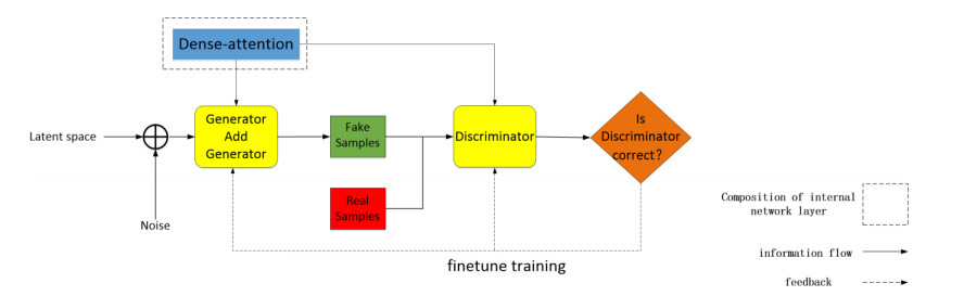
Protein engineering uses de novo protein design technology to change the protein gene sequence, and then improve the physical and chemical properties of proteins. These newly generated proteins will meet the needs of research better in properties and functions. The Dense-AutoGAN model is based on GAN, which is combined with an Attention mechanism to generate protein sequences. In this GAN architecture, the Attention mechanism and Encoder-decoder can improve the similarity of generated sequences and obtain variations in a smaller range on the original basis. Meanwhile, a new convolutional neural network is constructed by using the Dense. The dense network transmits in multiple layers over the generator network of the GAN architecture, which expands the training space and improves the effectiveness of sequence generation. Finally, the complex protein sequences are generated on the mapping of protein functions. Through comparisons of other models, the generated sequences of Dense-AutoGAN verify the model performance. The new generated proteins are highly accurate and effective in chemical and physical properties.

References

[1]	E. C. Alley, G. Khimulya, S. Biswas, M. AlQuraishi, G. M. Church, Unified rational protein engineering with sequence-based deep representation learning, Nat. Methods, 16 (2019), 1315–1322. https://doi.org/10.1038/s41592-019-0598-1 doi: 10.1038/s41592-019-0598-1
[2]	K. K. Yang, Z. Wu, F. H. Arnold, Machine-learning-guided directed evolution for protein engineering, Nat. Methods, 16 (2019), 687–694. https://doi.org/10.1038/s41592-019-0496-6 doi: 10.1038/s41592-019-0496-6
[3]	M. Rouhani, F. Khodabakhsh, D. Norouzian, R. A. Cohan, V. Valizadeh, Molecular dynamics simulation for rational protein engineering: Present and future prospectus, J. Mol. Graph. Model., 84 (2018), 43–53. https://doi.org/10.1016/j.jmgm.2018.06.009 doi: 10.1016/j.jmgm.2018.06.009
[4]	B. A. Meinen, C. D. Bahl, Breakthroughs in computational design methods open up new frontiers for de novo protein engineering, Protein Eng. Des. Sel., 34 (2021). https://doi.org/10.1093/protein/gzab007 doi: 10.1093/protein/gzab007
[5]	I. V. Korendovych, W. F. DeGrado, De novo protein design, a retrospective, Q. Rev. Biophys., 53 (2020). https://doi.org/10.1017/S0033583519000131 doi: 10.1017/S0033583519000131
[6]	E. Marcos, D. A. Silva, Essentials of de novo protein design: Methods and applications, WIREs Comput. Mol. Sci., 8 (2018), e1374. https://doi.org/10.1002/wcms.1374 doi: 10.1002/wcms.1374
[7]	Y. Hsia, R. Mout, W. Sheffler, N. I. Edman, I. Vulovic, Y. Park, et al., Design of multi-scale protein complexes by hierarchical building block fusion, Nat. Commun., 12 (2021), 1–10. https://doi.org/10.1038/s41467-021-22276-z doi: 10.1038/s41467-021-22276-z
[8]	J. O'Connell, Z. Li, J. Hanson, R. Heffernan, J. Lyons, K. Paliwal, et al., SPIN2: Predicting sequence profiles from protein structures using deep neural networks, Proteins: Struct. Function Bioinform., 86 (2018), 629–633. https://doi.org/10.1002/prot.25489 doi: 10.1002/prot.25489
[9]	Q. Zou, G. Lin, X. Jiang, X. Liu, X. Zeng, Sequence clustering in bioinformatics: An empirical study, Brief. Bioinform., 21 (2020), 1–10. https://doi.org/10.1093/bib/bby090 doi: 10.1093/bib/bby090
[10]	Y. Li, C. Huang, L. Ding, Z. Li, Y. Pan, X. Gao, Deep learning in bioinformatics: Introduction, application, and perspective in the big data era, Methods, 166 (2019), 4–21. https://doi.org/10.1016/j.ymeth.2019.04.008 doi: 10.1016/j.ymeth.2019.04.008
[11]	F. Gabler, S. Nam, S. Till, M. Mirdita, M. Steinegger, J. Söding, et al., Protein sequence analysis using the MPI bioinformatics toolkit, Curr. Protoc. Bioinform., 72 (2020), e108. https://doi.org/10.1002/cpbi.108 doi: 10.1002/cpbi.108
[12]	Kaitao Lai, Natalie Twine, Aidan O'Brien, Yi Guo, Denis Bauer, Artificial intelligence and machine learning in bioinformatics, Encycl. Bioinform. Comput. Biol., 1 (2019), 272–286. https://doi.org/10.1016/b978-0-12-809633-8.20325-7 doi: 10.1016/b978-0-12-809633-8.20325-7
[13]	Z. Qin, L. Wu, H. Sun, S. Huo, T. Ma, E. Lim, et al., Artificial intelligence method to design and fold alpha-helical structural proteins from the primary amino acid sequence, Extreme Mech. Lett., 36 (2020), 100652. https://doi.org/10.1016/j.eml.2020.100652 doi: 10.1016/j.eml.2020.100652
[14]	T. Kirioka, P. Aumpuchin, T. Kikuchi, Detection of folding sites of β-trefoil fold proteins based on amino acid sequence analyses and structure-based sequence alignment, J. Proteomics Bioinform., 10 (2017), 222–235. https://doi.org/10.4172/jpb.1000446 doi: 10.4172/jpb.1000446
[15]	B. Liu, BioSeq-Analysis: A platform for DNA, RNA and protein sequence analysis based on machine learning approaches, Brief. bioinform., 20 (2019), 1280–1294. https://doi.org/10.1093/bib/bbx165 doi: 10.1093/bib/bbx165
[16]	S. Makrodimitris, R. C. van Ham, M. J. Reinders, Improving protein function prediction using protein sequence and GO-term similarities, Bioinformatics, 35 (2019), 1116–1124. https://doi.org/10.1093/bioinformatics/bty751 doi: 10.1093/bioinformatics/bty751
[17]	Z. J. Lee, S. Su, C. Chuang, K. Liu, Genetic algorithm with ant colony optimization (GA-ACO) for multiple sequence alignment, Appl. Soft Comput., 8 (2008), 55–78. https://doi.org/10.1016/j.asoc.2006.10.012 doi: 10.1016/j.asoc.2006.10.012
[18]	M. Dorigo, M. Birattari, T. Stutzle, Ant colony optimization, IEEE Comput. Intell. Mag., 1 (2006), 28–39. https://doi.org/10.1109/MCI.2006.329691 doi: 10.1109/MCI.2006.329691
[19]	S. Katoch, S. S. Chauhan, V. Kumar, A review on genetic algorithm: Past, present, and future, Multimedia Tools Appl., 80 (2021), 8091–8126. https://doi.org/10.1007/s11042-020-10139-6 doi: 10.1007/s11042-020-10139-6
[20]	B. Bošković, J. Brest, Protein folding optimization using differential evolution extended with local search and component reinitialization, Inform. Sci., 454 (2018), 178–199. https://doi.org/10.1016/j.ins.2018.04.072 doi: 10.1016/j.ins.2018.04.072
[21]	M. Issa, A. E. Hassanien, D. Oliva, A. Helmi, I. Ziedana, A. Alzohairy, ASCA-PSO: Adaptive sine cosine optimization algorithm integrated with particle swarm for pairwise local sequence alignment, Expert Syst. Appl., 99 (2018), 56–70. https://doi.org/10.1016/j.eswa.2018.01.019 doi: 10.1016/j.eswa.2018.01.019
[22]	H. Nenavath, R. K. Jatoth, Hybridizing sine cosine algorithm with differential evolution for global optimization and object tracking, Appl. Soft Comput., 62 (2018), 1019–1043. https://doi.org/10.1016/j.asoc.2017.09.039 doi: 10.1016/j.asoc.2017.09.039
[23]	P. Dutta, S. Saha, S. Naskar, A multi-objective based PSO approach for inferring pathway activity utilizing protein interactions, Multimedia Tools Appl., 80 (2021), 30283–30303. https://doi.org/10.1007/s11042-020-09269-8 doi: 10.1007/s11042-020-09269-8
[24]	Q. Zhan, N. Wang, S. Jin, R. Tan, Q. Jiang, Y. Wang, Probpfp: A multiple sequence alignment algorithm combining partition function and hidden Markov model with particle swarm optimization, in 2018 IEEE International Conference on Bioinformatics and Biomedicine (BIBM), (2018), 1290–1295. https://doi.org/10.1109/BIBM.2018.8621220
[25]	H. Rademacher, On the partition function p (n), Proc. London Math. Soc., 2 (1938), 241–254. https://doi.org/10.1112/plms/s2-43.4.241 doi: 10.1112/plms/s2-43.4.241
[26]	N. Plattner, S. Doerr, G. de Fabritiis, F. Noé, Complete protein–protein association kinetics in atomic detail revealed by molecular dynamics simulations and Markov modelling, Nat. Chem., 9 (2017), 1005–1011. https://doi.org/10.1038/nchem.2785 doi: 10.1038/nchem.2785
[27]	C. Yang, Y. Lin, L. Chuang, H. Chang, A particle swarm optimization-based approach with local search for predicting protein folding, J. Comput. Biol., 24 (2017), 981–994. https://doi.org/10.1089/cmb.2016.0104 doi: 10.1089/cmb.2016.0104
[28]	M. F. M. Silva, L. F. Leijoto, C. N. Nobre, Algorithms analysis in adjusting the SVM parameters: An approach in the prediction of protein function, Appl. Artif. Intell., 31 (2017), 316–331. https://doi.org/10.1080/08839514.2017.1317207 doi: 10.1080/08839514.2017.1317207
[29]	Y. Ge, S. Zhao, X. Zhao, A step-by-step classification algorithm of protein secondary structures based on double-layer SVM model, Genomics, 112 (2020), 1941–1946. https://doi.org/10.1016/j.ygeno.2019.11.006 doi: 10.1016/j.ygeno.2019.11.006
[30]	K. C. Chou, L. Carlacci, Simulated annealing approach to the study of protein structures, Protein Eng. Des. Sel., 4 (1991), 661–667. https://doi.org/10.1093/protein/4.6.661 doi: 10.1093/protein/4.6.661
[31]	C. Yanover, M. Fromer, J.M. Shifman, Dead‐end elimination for multistate protein design, J. Comput. Chem., 28 (2007), 2122–2129. https://doi.org/10.1002/jcc.20661 doi: 10.1002/jcc.20661
[32]	A. W. Senior, R. Evans, J. Jumper, J. Kirkpatrick, L. Sifre, T. Green, et al., Improved protein structure prediction using potentials from deep learning, Nature, 577 (2020), 706–710. https://doi.org/10.1038/s41586-019-1923-7 doi: 10.1038/s41586-019-1923-7
[33]	M. Gao, J. Skolnick, A novel sequence alignment algorithm based on deep learning of the protein folding code, Bioinformatics, 37 (2021), 490–496. https://doi.org/10.1093/bioinformatics/btaa810 doi: 10.1093/bioinformatics/btaa810
[34]	M. Spencer, J. Eickholt, J. Cheng, A deep learning network approach to ab initio protein secondary structure prediction, IEEE/ACM Trans. Comput. Biol. Bioinform., 12 (2015), 103–112. https://doi.org/10.1109/TCBB.2014.2343960 doi: 10.1109/TCBB.2014.2343960
[35]	P. Kim, Convolutional neural network, in MATLAB Deep Learning, Springer, (2017), 121–147. https://doi.org/10.1007/978-1-4842-2845-6_6
[36]	J. Hou, B. Adhikari, J. Cheng, DeepSF: Deep convolutional neural network for mapping protein sequences to folds, Bioinformatics, 34 (2018), 1295–1303. https://doi.org/10.1093/bioinformatics/btx780 doi: 10.1093/bioinformatics/btx780
[37]	S. Wang, J. Peng, J. Ma, J. Xu, Protein secondary structure prediction using deep convolutional neural fields, Sci. Rep., 6 (2016), 1–11. https://doi.org/10.1038/srep18962 doi: 10.1038/srep18962
[38]	S. Wang, S. Weng, J. Ma, Q. Tang, DeepCNF-D: Predicting protein order/disorder regions by weighted deep convolutional neural fields, Int. J. Mol. Sci., 16 (2015), 17315–17330. https://doi.org/10.3390/ijms160817315 doi: 10.3390/ijms160817315
[39]	N. Killoran, L. J. Lee, A. Delong, D. Duvenaud, B. J. Frey, Generating and designing DNA with deep generative models, preprint, arXiv: 1712.06148v1. https://doi.org/10.48550/arXiv.1712.06148
[40]	E. Lin, C. H. Lin, H. Y. Lane, Relevant applications of generative adversarial networks in drug design and discovery: Molecular de novo design, dimensionality reduction, and de novo peptide and protein design, Molecules, 25 (2020), 3250. https://doi.org/10.3390/molecules25143250 doi: 10.3390/molecules25143250
[41]	C. Wan, D. T. Jones, Protein function prediction is improved by creating synthetic feature samples with generative adversarial networks, Nat. Mach. Intell., 2 (2020), 540–550. https://doi.org/10.1038/s42256-020-0222-1 doi: 10.1038/s42256-020-0222-1
[42]	A. Gupta, J. Zou, Feedback GAN for DNA optimizes protein functions, Nat. Mach. Intell., 1 (2019), 105–111. https://doi.org/10.1038/s42256-019-0017-4 doi: 10.1038/s42256-019-0017-4
[43]	M. R. Uddin, S. Mahbub, M. S. Rahman, M. S. Bayzid, SAINT: Self-attention augmented inception-inside-inception network improves protein secondary structure prediction, Bioinformatics, 36 (2020), 4599–4608.
[44]	G. Huang, Z. Liu, L. van der Maatene, K. Q. Weinberger, Densely connected convolutional networks. in 2017 IEEE Conference on Computer Vision and Pattern Recognition (CVPR), (2017). https://doi.org/10.1109/CVPR.2017.243
[45]	M. Steinegger, J. Söding, MMseqs2 enables sensitive protein sequence searching for the analysis of massive data sets, Nat. Biotechnol., 35 (2017), 1026–1028. https://doi.org/10.1038/nbt.3988 doi: 10.1038/nbt.3988
[46]	D. Repecka, V. Jauniskis, L. Karpus, E. Rembeza, I. Rokaitis, J. Zrimec, et al., Expanding functional protein sequence spaces using generative adversarial networks, Nat. Mach. Intell., 3 (2021), 324–333. https://doi.org/10.1038/s42256-021-00310-5 doi: 10.1038/s42256-021-00310-5
[47]	J. Jumper, R. Evans, A. Pritzel, T. Green, M. Figurnov, O. Ronneberger, et al., Highly accurate protein structure prediction with AlphaFold, Nature, 596 (2021), 583–589.

Reader Comments

Your name:*

Email:*
© 2023 the Author(s), licensee AIMS Press. This is an open access article distributed under the terms of the Creative Commons Attribution License (http://creativecommons.org/licenses/by/4.0)