Flexible ku/k band frequency reconfigurable bandpass filter

Ambati. Navya; Govardhani. Immadi; Madhavareddy. Venkata Narayana; Ambati. Navya; Govardhani. Immadi; Madhavareddy. Venkata Narayana

doi:10.3934/electreng.2022002

AIMS Electronics and Electrical Engineering

2022, Volume 6, Issue 1: 16-28. doi: 10.3934/electreng.2022002

Previous Article Next Article

Research article Special Issues

Flexible ku/k band frequency reconfigurable bandpass filter

Department of ECE, KLEF, Vaddeswaram, Guntur, Andhra Pradesh, India
Academic editor: Reza K. Amineh

Received: 09 November 2021 Revised: 21 December 2021 Accepted: 06 January 2022 Published: 13 January 2022

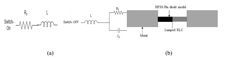
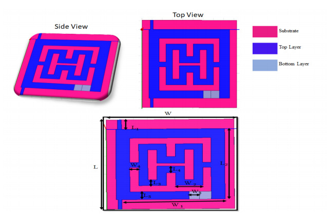
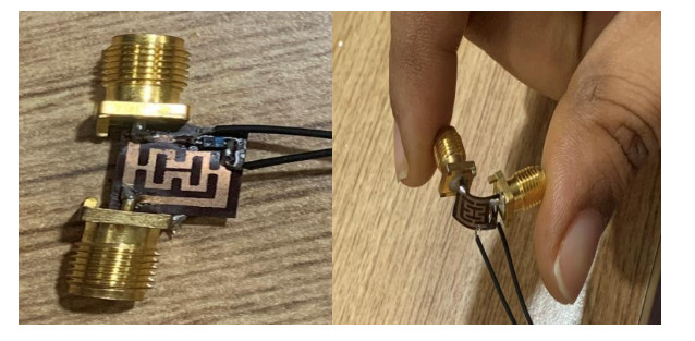
The proposed reconfigurable BPF satisfies the International Telecommunication Unionos (ITU) region 3 spectrum requirement. In transmit mode, the frequency range 11.41-12.92 GHz is used by the direct broadcast service (DBS) and the fixed satellite service (FSS). Direct broadcast service (DBS) in reception mode employs 11.7-12.2 GHz and 17.3-17.8 GHz frequency ranges. Frequency reconfigurable filters are popular because they can cover wide range of frequencies, reducing system cost and space. Another emerging trend is electronic component flexibility or conformability, which allows them to be mounted on non-planar objects and are used in wearable applications. This project contains a frequency-reconfigurable BPF that has been entirely printed on a flexible polimide substrate. Frequency reconfigurability is obtained by using a pin diode HSCH 5318 and it is used to switch between 12 GHz and 18 GHz. The prototype reconfigurable BPF is highly compact and low-cost due to the flexible polimide substrate and the measured results are promising and match the simulated results well.
- reconfigurable filter,
- HFSS,
- bandpass filter,
- switch, frequency
Citation: Ambati. Navya, Govardhani. Immadi, Madhavareddy. Venkata Narayana. Flexible ku/k band frequency reconfigurable bandpass filter[J]. AIMS Electronics and Electrical Engineering, 2022, 6(1): 16-28. doi: 10.3934/electreng.2022002

Related Papers:

Abstract

The proposed reconfigurable BPF satisfies the International Telecommunication Unionos (ITU) region 3 spectrum requirement. In transmit mode, the frequency range 11.41-12.92 GHz is used by the direct broadcast service (DBS) and the fixed satellite service (FSS). Direct broadcast service (DBS) in reception mode employs 11.7-12.2 GHz and 17.3-17.8 GHz frequency ranges. Frequency reconfigurable filters are popular because they can cover wide range of frequencies, reducing system cost and space. Another emerging trend is electronic component flexibility or conformability, which allows them to be mounted on non-planar objects and are used in wearable applications. This project contains a frequency-reconfigurable BPF that has been entirely printed on a flexible polimide substrate. Frequency reconfigurability is obtained by using a pin diode HSCH 5318 and it is used to switch between 12 GHz and 18 GHz. The prototype reconfigurable BPF is highly compact and low-cost due to the flexible polimide substrate and the measured results are promising and match the simulated results well.

References

[1]	Arain S, Vryonides P, Abbasi M, et al. (2018) Reconfigurable bandwidth bandpass filter with enhanced out-of-band rejection using π-section loaded ring resonator. IEEE Microw Wirel Co 28: 28-30. https://doi.org/10.1109/LMWC.2017.2776212 doi: 10.1109/LMWC.2017.2776212
[2]	Cheng T, Tam K (2017) A wideband bandpass filter with reconfigurable bandwidth based on cross-shaped resonator. IEEE Microw Wirel Co 27: 909-91. https://doi.org/10.1109/LMWC.2017.2746679 doi: 10.1109/LMWC.2017.2746679
[3]	Zhang X, Wong S, Guo S, et al. (2020) Design of notched-wideband bandpass filters with reconfigurable bandwidth based on terminated cross-shaped resonators. IEEE Access 8: 37416-37427. https://doi.org/10.1109/ACCESS.2020.2975379 doi: 10.1109/ACCESS.2020.2975379
[4]	Sanchez-Soriano MA, Gomez-Garcia R, Torregrosa-Penalva G, et al. (2013) Reconfigurable-bandwidth bandpass filter within 10-50%. IET Microw Antenna P 7: 502-509. https://doi.org/10.1049/iet-map.2012.0274 doi: 10.1049/iet-map.2012.0274
[5]	Borja AL, Carbonell J, Martinez JL, et al. (2011) A controllable bandwidth filter using varactor-loaded metamaterial-inspired transmission lines. IEEE Antenn Wirel Pr 10: 1575-1578. https://doi.org/10.1109/LAWP.2012.2183111 doi: 10.1109/LAWP.2012.2183111
[6]	Chen N, Jeng SK (2012) Reconfigurable bandpass filter with separately relocatable passband edge. IEEE Microw Wirel Co 22: 559-561. https://doi.org/10.1109/LMWC.2012.2225606 doi: 10.1109/LMWC.2012.2225606
[7]	Wang XM, Bi XK, Guo SH, et al. (2020) Synthesis design of equal-ripple and quasi-elliptic wideband BPFs with independently reconfigurable lower passband edge. IEEE Access 8: 76856-76866. https://doi.org/10.1109/ACCESS.2020.2989449 doi: 10.1109/ACCESS.2020.2989449
[8]	Gomez-Garcia R, Guyette AC, Psychogiou D, et al. (2019) Quasi-elliptic multi-band filters with center-frequency and bandwidth tenability. IEEE Microw Wirel Co 26: 192-194. https://doi.org/10.1109/LMWC.2016.2526026 doi: 10.1109/LMWC.2016.2526026
[9]	Huang BC, Chen NW, Jeng SK (2014) A reconfigurable bandpass filter based on a varactor-perturbed, T-shaped dual-mode resonator. IEEE Microw Wirel Co 24: 297-299. https://doi.org/10.1109/LMWC.2014.2306893 doi: 10.1109/LMWC.2014.2306893
[10]	Sanchez-Renedo M, Gomez-Garcia R, Alonso JI, et al. (2005) Tunable combline filter with continuous control of center frequency and bandwidth. IEEE T Microw Theory 53: 191-199. https://doi.org/10.1109/TMTT.2004.839309 doi: 10.1109/TMTT.2004.839309
[11]	Wong PW, Hunter IC (2009) Electronically reconfigurable microwave bandpass filter. IEEE T Microw Theory 57: 3070-3079. https://doi.org/10.1109/TMTT.2009.2033883 doi: 10.1109/TMTT.2009.2033883
[12]	Tsai H, Chen N, Jeng S (2013) Center frequency and bandwidth controllable microstrip bandpass filter design using loop-shaped dual-mode resonator. IEEE T Microw Theory 61: 3590-3600. https://doi.org/10.1109/TMTT.2013.2280129 doi: 10.1109/TMTT.2013.2280129
[13]	Guo H, Hong J (2018) Varactor-tuned dual-mode bandpass filter with nonuniform Q distribution. IEEE Microw Wirel Co 28: 1002-1004. https://doi.org/10.1109/LMWC.2018.2870934 doi: 10.1109/LMWC.2018.2870934
[14]	Schuster C, Wiens A, Schmidt F, et al. (2017) Performance analysis of reconfigurable bandpass filters with continuously tunable center frequency and bandwidth. IEEE T Microw Theory 65: 4572-4583. https://doi.org/10.1109/TMTT.2017.2742479 doi: 10.1109/TMTT.2017.2742479
[15]	Kingsly S, Kanagasabai M, Alsath MG, et al. (2018) Compact frequency and bandwidth tunable bandpass-band stop microstrip filter. IEEE Microw Wirel Co 28: 786-788. https://doi.org/10.1109/LMWC.2018.2858005 doi: 10.1109/LMWC.2018.2858005
[16]	Ghaderi A, Golestanifar A, Shama F (2017) Design of a compact microstrip tunable dual-band bandpass filter. AEU-Int J Electron C 82: 391-396. https://doi.org/10.1016/j.aeue.2017.10.002 doi: 10.1016/j.aeue.2017.10.002
[17]	Qin W, Cai J, Li YL, et al. (2017) Wideband tunable bandpass filter using optimized varactor-loaded SIRs. IEEE Microw Wirel Co 27: 812-814. https://doi.org/10.1109/LMWC.2017.2734848 doi: 10.1109/LMWC.2017.2734848
[18]	Karim MF, Guo YX, Chen ZN, et al. (2009) Miniaturized reconfigurable and switchable filter from UWB to 2.4 GHz WLAN using PIN diodes. In IEEE Microwave Symposium Digest. MTT-S International, 509-512. https://doi.org/10.1109/MWSYM.2009.5165745
[19]	Elelimy AM, El-Tager AM, Sobih AG (2013) A compact size switched reconfigurable tri-band BPF for modern wireless applications. In 56th International Midwest Symposium on Circuits and Systems (MWSCAS), 772-775. https://doi.org/10.1109/MWSCAS.2013.6674763
[20]	Boutejdar A (2016) Design of 5 GHz-compact reconfigurable DGS-bandpass filter using varactor-diode device and coupling matrix technique. Microw Opt Techn Let 58: 304-309. https://doi.org/10.1002/mop.29561 doi: 10.1002/mop.29561
[21]	Zhang ZC, Liu H (2018) A ultra-compact wideband bandpass filter using a quad mode stub-loaded resonator. Prog Electrom Res Le 77: 35-40.
[22]	Navya A, Immadi G, Narayana MV (2021) A Low-Profile Wideband BPF for Ku Band Applications, Prog Electrom Res Le 100: 127-135. https://doi.org/10.2528/PIERL21082101 doi: 10.2528/PIERL21082101
[23]	Ambati N, Immadi G, Narayana MV, et al. (2021), Parametric Analysis of the Defected Ground Structure-Based Hairpin Band Pass Filter for VSAT System on Chip Applications. Eng Technol Appl Sci 11: 7892-7896. https://doi.org/10.48084/etasr.4495 doi: 10.48084/etasr.4495

Reader Comments

Your name:*

Email:*
© 2022 the Author(s), licensee AIMS Press. This is an open access article distributed under the terms of the Creative Commons Attribution License (http://creativecommons.org/licenses/by/4.0)