The convolutional neural network, as the backbone network for medical image segmentation, has shown good performance in the past years. However, its drawbacks cannot be ignored, namely, convolutional neural networks focus on local regions and are difficult to model global contextual information. For this reason, transformer, which is used for text processing, was introduced into the field of medical segmentation, and thanks to its expertise in modelling global relationships, the accuracy of medical segmentation was further improved. However, the transformer-based network structure requires a certain training set size to achieve satisfactory segmentation results, and most medical segmentation datasets are small in size. Therefore, in this paper we introduce a gated position-sensitive axial attention mechanism in the self-attention module, so that the transformer-based network structure can also be adapted to the case of small datasets. The common operation of the visual transformer introduced to visual processing when dealing with segmentation tasks is to divide the input image into equal patches of the same size and then perform visual processing on each patch, but this simple division may lead to the destruction of the structure of the original image, and there may be large unimportant regions in the divided grid, causing attention to stay on the uninteresting regions, affecting the segmentation performance. Therefore, in this paper, we add iterative sampling to update the sampling positions, so that the attention stays on the region to be segmented, reducing the interference of irrelevant regions and further improving the segmentation performance. In addition, we introduce the strip convolution module (SCM) and pyramid pooling module (PPM) to capture the global contextual information. The proposed network is evaluated on several datasets and shows some improvement in segmentation accuracy compared to networks of recent years.
Citation: Shen Jiang, Jinjiang Li, Zhen Hua. Transformer with progressive sampling for medical cellular image segmentation[J]. Mathematical Biosciences and Engineering, 2022, 19(12): 12104-12126. doi: 10.3934/mbe.2022563
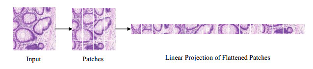
The convolutional neural network, as the backbone network for medical image segmentation, has shown good performance in the past years. However, its drawbacks cannot be ignored, namely, convolutional neural networks focus on local regions and are difficult to model global contextual information. For this reason, transformer, which is used for text processing, was introduced into the field of medical segmentation, and thanks to its expertise in modelling global relationships, the accuracy of medical segmentation was further improved. However, the transformer-based network structure requires a certain training set size to achieve satisfactory segmentation results, and most medical segmentation datasets are small in size. Therefore, in this paper we introduce a gated position-sensitive axial attention mechanism in the self-attention module, so that the transformer-based network structure can also be adapted to the case of small datasets. The common operation of the visual transformer introduced to visual processing when dealing with segmentation tasks is to divide the input image into equal patches of the same size and then perform visual processing on each patch, but this simple division may lead to the destruction of the structure of the original image, and there may be large unimportant regions in the divided grid, causing attention to stay on the uninteresting regions, affecting the segmentation performance. Therefore, in this paper, we add iterative sampling to update the sampling positions, so that the attention stays on the region to be segmented, reducing the interference of irrelevant regions and further improving the segmentation performance. In addition, we introduce the strip convolution module (SCM) and pyramid pooling module (PPM) to capture the global contextual information. The proposed network is evaluated on several datasets and shows some improvement in segmentation accuracy compared to networks of recent years.

| [1] | J. Devlin, M. W. Chang, K. Lee, K. Toutanova, Bert: Pre-training of deep bidirectional transformers for language understanding, preprint, arXiv: 1810.04805. https://doi.org/10.48550/arXiv.1810.04805 |
| [2] | A. Vaswani, N. Shazeer, N. Parmar, J. Uszkoreit, L. Jones, A. N. Gomez, et al., Attention is all you need, Adv. Neural Inf. Process. Syst., 30 (2017). |
| [3] | H. Wang, Y. Zhu, B. Green, H. Adam, A. Yuille, L. C. Chen, Axial-Deeplab: Stand-alone axial-attention for panoptic segmentation, in European Conference on Computer Vision, (2020), 108–126. https://doi.org/10.1007/978-3-030-58548-8 |
| [4] | M. Chen, A. Radford, R. Child, J. Wu, H. Jun, D. Luan, et al., Generative pretraining from pixels, in International Conference on Machine Learning, (2020), 1691–1703. |
| [5] | A. Dosovitskiy, L. Beyer, A. Kolesnikov, D. Weissenborn, X. Zhai, T. Unterthiner, et al., An image is worth 16x16 words: Transformers for image recognition at scale, preprint, arXiv: 2010.11929. https://doi.org/10.48550/arXiv.2010.11929 |
| [6] | X. Zhu, W. Su, L. Lu, B. Li, X. Wang, J. Dai, Deformable detr: Deformable transformers for end-to-end object detection, preprint, arXiv: 2010.04159. https://doi.org/10.48550/arXiv.2010.04159 |
| [7] | M. Zheng, P. Gao, R. Zhang, K. Li, X. Wang, H. Li, et al., End-to-end object detection with adaptive clustering transformer, preprint, arXiv: 2011.09315. https://doi.org/10.48550/arXiv.2011.09315 |
| [8] | Z. Dai, B. Cai, Y. Lin, J. Chen, Up-detr: Unsupervised pre-training for object detection with transformers, in Proceedings of the IEEE/CVF Conference on Computer Vision and Pattern Recognition, (2021), 1601–1610. https://doi.org/10.1109/CVPR46437.2021.00165 |
| [9] | Z. Sun, S. Cao, Y. Yang, K. M. Kitani, Rethinking transformer-based set prediction for object detection, in Proceedings of the IEEE/CVF International Conference on Computer Vision, (2021), 3611–3620. https://doi.org/10.1109/ICCV48922.2021.00359 |
| [10] |
Z. An, X. Wang, B. Li, Z. Xiang, B. Zhang, Robust visual tracking for uavs with dynamic feature weight selection, Appl. Intell., 2022 (2022), 1–14. https://doi.org/10.1007/s10489-022-03719-6 doi: 10.1007/s10489-022-03719-6

|
| [11] |
R. Muthukrishnan, M. Radha, Edge detection techniques for image segmentation, Int. J. Comput. Sci. Inf. Technol., 3 (2011), 259. https://doi.org/10.5121/ijcsit.2011.3620 doi: 10.5121/ijcsit.2011.3620
|
| [12] |
N. Otsu, A threshold selection method from gray-level histograms, IEEE Trans. Syst. Man Cybern., 9 (1979), 62–66. https://doi.org/10.1109/TSMC.1979.4310076 doi: 10.1109/TSMC.1979.4310076
|
| [13] | H. G. Kaganami, Z. Beiji, Region-based segmentation versus edge detection, in 2009 Fifth International Conference on Intelligent Information Hiding and Multimedia Signal Processing, (2009), 1217–1221. https://doi.org/10.1109/IIH-MSP.2009.13 |
| [14] |
M. Kass, A. Witkin, D. Terzopoulos, Snakes: Active contour models, Int. J. Comput. Vision, 1 (1988), 321–331. https://doi.org/10.1007/BF00133570 doi: 10.1007/BF00133570
|
| [15] | O. Ronneberger, P. Fischer, T. Brox, U-net: Convolutional networks for biomedical image segmentation, in International Conference on Medical Image Computing and Computer-Assisted Intervention, (2015), 234–241. https://doi.org/10.1007/978-3-319-24574-4 |
| [16] |
X. Li, H. Chen, X. Qi, Q. Dou, C. W. Fu, P. A. Heng, H-denseunet: Hybrid densely connected unet for liver and tumor segmentation from ct volumes, IEEE Trans. Med. Imaging, 37 (2018), 2663–2674. https://doi.org/10.1109/TMI.2018.2845918 doi: 10.1109/TMI.2018.2845918
|
| [17] | O. Oktay, J. Schlemper, L. L. Folgoc, M. Lee, M. Heinrich, K. Misawa, et al., Attention u-net: Learning where to look for the pancreas, preprint, arXiv: 1804.03999. https://doi.org/10.48550/arXiv.1804.03999 |
| [18] | X. Xiao, S. Lian, Z. Luo, S. Li, Weighted res-unet for high-quality retina vessel segmentation, in 2018 9th International Conference on Information Technology in Medicine and Education (ITME), (2018), 327–331. https://doi.org/10.1109/ITME.2018.00080 |
| [19] | Z. Zhou, M. M. Rahman-Siddiquee, N. Tajbakhsh, J. Liang, Unet++: A nested u-net architecture for medical image segmentation, in Deep Learning in Medical Image Analysis and Multimodal Learning for Clinical Decision Support, (2018), 3–11. https://doi.org/10.1007/978-3-030-00889-5 |
| [20] | M. Z. Alom, M. Hasan, C. Yakopcic, T. M. Taha, V. K. Asari, Recurrent residual convolutional neural network based on u-net (r2u-net) for medical image segmentation, preprint, arXiv: 1802.06955. https://doi.org/10.48550/arXiv.1802.06955 |
| [21] | Ö. Çiçek, A. Abdulkadir, S. S. Lienkamp, T. Brox, O. Ronneberger, 3D u-net: Learning dense volumetric segmentation from sparse annotation, in International Conference on Medical Image Computing and Computer-Assisted Intervention, (2016), 424–432. https://doi.org/10.1007/978-3-319-46723-8_49 |
| [22] |
C. Zhao, Y. Xu, Z. He, J. Tang, Y. Zhang, J. Han, et al., Lung segmentation and automatic detection of covid-19 using radiomic features from chest CT images, Pattern Recognit., 119 (2021), 108071. 2021. https://doi.org/10.1016/j.patcog.2021.108071 doi: 10.1016/j.patcog.2021.108071
|
| [23] |
X. Liu, A. Yu, X. Wei, Z. Pan, J. Tang, Multimodal mr image synthesis using gradient prior and adversarial learning, IEEE J. Sel. Top. Signal Process., 14 (2020), 1176–1188. https://doi.org/10.1109/JSTSP.2020.3013418 doi: 10.1109/JSTSP.2020.3013418
|
| [24] |
X. Liu, Q. Yuan, Y. Gao, K. He, S. Wang, X. Tang, et al., Weakly supervised segmentation of covid19 infection with scribble annotation on CT images, Pattern Recognit., 122 (2022), 108341. https://doi.org/10.1016/j.patcog.2021.108341 doi: 10.1016/j.patcog.2021.108341
|
| [25] |
J. He, Q. Zhu, K. Zhang, P. Yu, J. Tang, An evolvable adversarial network with gradient penalty for covid-19 infection segmentation, Appl. Soft Comput., 113 (2021), 107947. https://doi.org/10.1016/j.asoc.2021.107947 doi: 10.1016/j.asoc.2021.107947
|
| [26] |
N. Mu, H. Wang, Y. Zhang, J. Jiang, J. Tang, Progressive global perception and local polishing network for lung infection segmentation of covid-19 ct images, Pattern Recognit., 120 (2021), 108168. https://doi.org/10.1016/j.patcog.2021.108168 doi: 10.1016/j.patcog.2021.108168
|
| [27] |
L. C. Chen, G. Papandreou, I. Kokkinos, K. Murphy, A. L. Yuille, Deeplab: Semantic image segmentation with deep convolutional nets, atrous convolution, and fully connected crfs, IEEE Trans. Pattern Anal. Mach. Intell., 40 (2017), 834–848. https://doi.org/10.1109/TPAMI.2017.2699184 doi: 10.1109/TPAMI.2017.2699184
|
| [28] | W. Wang, E. Xie, X. Li, D. P. Fan, K. Song, D. Liang, et al., Pyramid vision transformer: A versatile backbone for dense prediction without convolutions, in Proceedings of the IEEE/CVF International Conference on Computer Vision, (2021), 568–578. https://doi.org/10.1109/ICCV48922.2021.00061 |
| [29] | H. H. Newman, F. N. Freeman, K. J. Holzinger, Twins: A study of Heredity and Environment, Univ. Chicago Press, 1937. |
| [30] | Z. Liu, Y. Lin, Y. Cao, H. Hu, Y. Wei, Z. Zhang, et al., Swin transformer: Hierarchical vision transformer using shifted windows, in Proceedings of the IEEE/CVF International Conference on Computer Vision, (2021), 10012–10022. https://doi.org/10.1109/ICCV48922.2021.00986 |
| [31] | J. M. J. Valanarasu, P. Oza, I. Hacihaliloglu, V. M. Patel, Medical transformer: Gated axial-attention for medical image segmentation, in International Conference on Medical Image Computing and Computer-Assisted Intervention, (2021), 36–46. https://doi.org/10.1007/978-3-030-87193-2 |
| [32] |
R. Meleppat, M. Matham, L. Seah, An efficient phase analysis-based wavenumber linearization scheme for swept source optical coherence tomography systems, Laser Phys. Lett., 12 (2015), 055601. https://doi.org/10.1088/1612-2011/12/5/055601 doi: 10.1088/1612-2011/12/5/055601
|
| [33] | R. K. Meleppat, E. B. Miller, S. K. Manna, P. Zhang, E. N. Pugh Jr, R. J. Zawadzki, Multiscale hessian filtering for enhancement of OCT angiography images, in Ophthalmic Technologies XXIX, 10858 (2019), 64–70. https://doi.org/10.1117/12.2511044 |
| [34] |
R. K. Meleppat, K. E. Ronning, S. J. Karlen, M. E. Burns, E. N. Pugh, R. J. Zawadzki, In vivo multimodal retinal imaging of disease-related pigmentary changes in retinal pigment epithelium, Sci. Rep., 11 (2021), 1–14. https://doi.org/10.1038/s41598-021-95320-z doi: 10.1038/s41598-021-95320-z
|
| [35] | R. K. Meleppat, M. V. Matham, L. K. Seah, Optical frequency domain imaging with a rapidly swept laser in the 1300nm bio-imaging window, in International Conference on Optical and Photonic Engineering (icOPEN 2015), 9524 (2015), 721–729. https://doi.org/10.1117/12.2190530 |
| [36] | H. Zhao, J. Shi, X. Qi, X. Wang, J. Jia, Pyramid scene parsing network, in Proceedings of the IEEE conference on computer vision and pattern recognition, (2017), 2881–2890. https://doi.org/10.1109/CVPR.2017.660 |
| [37] |
J. Mei, R. J. Li, W. Gao, M. M. Cheng, Coanet: Connectivity attention network for road extraction from satellite imagery, IEEE Trans. Image Process., 30 (2021), 8540–8552. https://doi.org/10.1109/TIP.2021.3117076 doi: 10.1109/TIP.2021.3117076
|
| [38] | X. Yue, S. Sun, Z. Kuang, M. Wei, P. H. Torr, W. Zhang, et al., Vision transformer with progressive sampling, in Proceedings of the IEEE/CVF International Conference on Computer Vision, (2021), 387–396. https://doi.org/10.1109/ICCV48922.2021.00044 |
| [39] |
K. Sirinukunwattana, J. P. Pluim, H. Chen, X. Qi, P. A. Heng, Y. B. Guo, et al., Gland segmentation in colon histology images: The glas challenge contest, Med. Image Anal., 35 (2017), 489–502. https://doi.org/10.1016/j.media.2016.08.008 doi: 10.1016/j.media.2016.08.008
|
| [40] |
N. Kumar, R. Verma, D. Anand, Y. Zhou, O. F. Onder, E. Tsougenis, et al., A multi-organ nucleus segmentation challenge, IEEE Trans. Med. Imaging, 39 (2019), 1380–1391. https://doi.org/10.1109/TMI.2019.2947628 doi: 10.1109/TMI.2019.2947628
|
| [41] |
N. Kumar, R. Verma, S. Sharma, S. Bhargava, A. Vahadane, A. Sethi, A dataset and a technique for generalized nuclear segmentation for computational pathology, IEEE Trans. Med. Imaging, 36 (2017), 1550–1560. https://doi.org/10.1109/TMI.2017.2677499 doi: 10.1109/TMI.2017.2677499
|
| [42] |
J. Bernal, F. J. Sánchez, G. Fernández-Esparrach, D. Gil, C. Rodríguez, F. Vilariño, Wm-dova maps for accurate polyp highlighting in colonoscopy: Validation vs. saliency maps from physicians, Comput. Med. Imaging Graphics, 43 (2015), 99–111. https://doi.org/10.1016/j.compmedimag.2015.02.007 doi: 10.1016/j.compmedimag.2015.02.007
|
| [43] |
J. M. J. Valanarasu, V. A. Sindagi, I. Hacihaliloglu, V. M. Patel, Kiu-net: Overcomplete convolutional architectures for biomedical image and volumetric segmentation, IEEE Transa. Med. Imaging, 41 (2021), 965–976. https://doi.org/10.1109/TMI.2021.3130469 doi: 10.1109/TMI.2021.3130469
|
| [44] |
Y. Chen, K. Wang, X. Liao, Y. Qian, Q. Wang, Z. Yuan, et al., Channel-unet: A spatial channel-wise convolutional neural network for liver and tumors segmentation, Front. Genet., 10 (2019), 1110. https://doi.org/10.3389/fgene.2019.01110 doi: 10.3389/fgene.2019.01110
|
| [45] | N. Chinchor, B. M. Sundheim, Muc-5 evaluation metrics, in Fifth Message Understanding Conference (MUC-5): Proceedings of a Conference Held in Baltimore, Maryland, 1993. https://doi.org/10.3115/1072017.1072026 |
| [46] | S. Niwattanakul, J. Singthongchai, E. Naenudorn, S. Wanapu, Using of jaccard coefficient for keywords similarity, in Proceedings of the International Multiconference of Engineers and Computer Scientists, 1 (2013), 380–384. |


Figures(12) / Tables(5)

Shen Jiang, Jinjiang Li, Zhen Hua. Transformer with progressive sampling for medical cellular image segmentation[J]. Mathematical Biosciences and Engineering, 2022, 19(12): 12104-12126. doi: 10.3934/mbe.2022563


 DownLoad: