Wading bird foraging on a wetland landscape: a comparison of two strategies

Hyo Won Lee; Donald L. DeAngelis; Simeon Yurek; Stephen Tennenbaum; Hyo Won Lee; Donald L. DeAngelis; Simeon Yurek; Stephen Tennenbaum

doi:10.3934/mbe.2022361

Mathematical Biosciences and Engineering

2022, Volume 19, Issue 8: 7687-7718. doi: 10.3934/mbe.2022361

Previous Article Next Article

Research article Special Issues

Wading bird foraging on a wetland landscape: a comparison of two strategies

1.
Biological Sciences Department, Florida International University, Miami, FL, USA
2.
U.S. Geological Survey, Wetland and Aquatic Research Center, Davie, FL 33314, USA
3.
U.S. Geological Survey, Wetland and Aquatic Research Center, Gainesville, FL 32653, USA

Academic Editor: Yang Kuang

Received: 08 March 2022 Revised: 01 May 2022 Accepted: 07 May 2022 Published: 24 May 2022

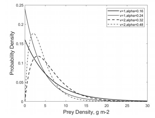
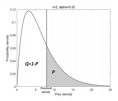
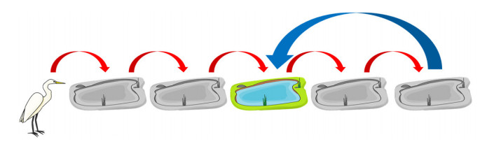
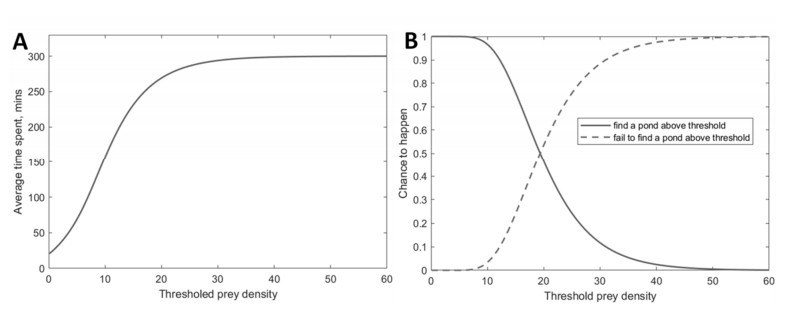
Tactile-feeding wading birds, such as wood storks and white ibises, require high densities of prey such as small fishes and crayfish to support themselves and their offspring during the breeding season. Prey availability in wetlands is often determined by seasonal hydrologic pulsing, such as in the subtropical Everglades, where spatial distributions of prey can vary through time, becoming heterogeneously clumped in patches, such as ponds or sloughs, as the wetland dries out. In this mathematical modeling study, we selected two possible foraging strategies to examine how they impact total energetic intake over a time scale of one day. In the first, wading birds sample prey patches without a priori knowledge of the patches' prey densities, moving from patch to patch, staying long enough to estimate the prey density, until they find one that meets a predetermined satisfactory threshold, and then staying there for a longer period. For this case, we solve for a wading bird's expected prey intake over the course of a day, given varying theoretical probability distributions of patch prey densities across the landscape. In the second strategy considered, it is assumed that the wading bird samples a given number of patches, and then uses memory to return to the highest quality patch. Our results show how total intake over a day is impacted by assumptions of the parameters governing the spatial distribution of prey among patches, which is a key source of parameter uncertainty in both natural and managed ecosystems. Perhaps surprisingly, the foraging strategy that uses a prey density threshold generally led to higher maximum potential prey intake than the strategy for using memory to return to the best patch sampled. These results will contribute to understanding the foraging of wading birds and to the management of wetlands.
- prey density probability distribution,
- heterogeneous landscape,
- threshold for foraging,
- foraging using memory
Citation: Hyo Won Lee, Donald L. DeAngelis, Simeon Yurek, Stephen Tennenbaum. Wading bird foraging on a wetland landscape: a comparison of two strategies[J]. Mathematical Biosciences and Engineering, 2022, 19(8): 7687-7718. doi: 10.3934/mbe.2022361

Related Papers:

Abstract

Tactile-feeding wading birds, such as wood storks and white ibises, require high densities of prey such as small fishes and crayfish to support themselves and their offspring during the breeding season. Prey availability in wetlands is often determined by seasonal hydrologic pulsing, such as in the subtropical Everglades, where spatial distributions of prey can vary through time, becoming heterogeneously clumped in patches, such as ponds or sloughs, as the wetland dries out. In this mathematical modeling study, we selected two possible foraging strategies to examine how they impact total energetic intake over a time scale of one day. In the first, wading birds sample prey patches without a priori knowledge of the patches' prey densities, moving from patch to patch, staying long enough to estimate the prey density, until they find one that meets a predetermined satisfactory threshold, and then staying there for a longer period. For this case, we solve for a wading bird's expected prey intake over the course of a day, given varying theoretical probability distributions of patch prey densities across the landscape. In the second strategy considered, it is assumed that the wading bird samples a given number of patches, and then uses memory to return to the highest quality patch. Our results show how total intake over a day is impacted by assumptions of the parameters governing the spatial distribution of prey among patches, which is a key source of parameter uncertainty in both natural and managed ecosystems. Perhaps surprisingly, the foraging strategy that uses a prey density threshold generally led to higher maximum potential prey intake than the strategy for using memory to return to the best patch sampled. These results will contribute to understanding the foraging of wading birds and to the management of wetlands.

References

[1]	R. Liu, S. A. Gourley, D. L. DeAngelis, J. P. Bryant, Modeling the dynamics of woody plant–herbivore interactions with age-dependent toxicity, J. Math. Biol, 65 (2012), 521–552. https://doi.org/10.1007/s00285-011-0470-0 doi: 10.1007/s00285-011-0470-0
[2]	R. Liu, S. A. Gourley, D. L. DeAngelis, J. P. Bryant, A mathematical model of woody plant chemical defenses and snowshoe hare feeding behavior in boreal forests: the effect of age-dependent toxicity of twig segments, SIAM J. Appl. Math., 73 (2013), 281–304. https://doi.org/10.1137/110848219 doi: 10.1137/110848219
[3]	D. L. DeAngelis, J. P. Bryant, R. Liu, S. A. Gourley, C. J. Krebs, P. B Reichardt, A plant toxin mediated mechanism for the lag in snowshoe hare population recovery following cyclic declines, Oikos, 124 (2015), 796–805. https://doi.org/10.1111/oik.01671 doi: 10.1111/oik.01671
[4]	S. A. Gourley, R. Liu, J. Wu, Spatiotemporal distributions of migratory birds: Patchy models with delay, SIAM J. Appl. Dyn. Syst., 9 (2010), 589–610. https://doi.org/10.1137/090767261 doi: 10.1137/090767261
[5]	G. T. Bancroft, A. M. Strong, R. J. Sawicki, W. Hoffman, S. D. Jewell, Relationship among wading bird foraging patterns, colony locations, and hydrology in the Everglades, St. Lucie Press, (1994), 615–665. Available from: https://www.taylorfrancis.com/chapters/edit/10.1201/9781466571754-34.
[6]	J. C. Ogden, A comparison of wading bird nesting colony dynamics (1931–1946 and 1974–1989) as an indication of ecosystem conditions in the Southern Everglades, St. Lucie Press, (1994), 533–570. Available from: https://www.taylorfrancis.com/chapters/edit/10.1201/9781466571754-34.
[7]	E. L. Charnov, Optimal foraging: attack strategy of a mantid, Am. Nat., 110 (1976), 141–151. https://doi.org/10.1086/283054 doi: 10.1086/283054
[8]	D. W. Stephens, J. R. Krebs, Foraging theory, Princeton University Press, 2019. https://doi.org/10.1515/9780691206790
[9]	D. L. DeAngelis, S. Yurek, S. Tennenbaum, H. W. Lee, Hierarchical functional response of a forager on a wetland landscape, Front. Ecol. Evol., (2021), 655. https://doi.org/10.3389/fevo.2021.729236 doi: 10.3389/fevo.2021.729236
[10]	E. A. Adams, P. C. Frederick, Effects of methylmercury and spatial complexity on foraging behavior and foraging efficiency in juvenile white ibises (Eudocimus albus), Environ. Toxicol. Chem., 27 (2009), 1708–1712. https://doi.org/10.1897/07-466.1 doi: 10.1897/07-466.1
[11]	J. P. Royston, Algorithm AS 177: Expected normal order statistics (exact and approximate), J. R. Stat. Soc., Ser. C (Appl. Stat.), 31 (1982), 161–165. https://doi.org/10.2307/2347982 doi: 10.2307/2347982
[12]	J. A. Kushlan, Population energetics of the American white ibis, The Auk, 94 (1977), 114–122. https://doi.org/10.1093/auk/94.1.114 doi: 10.1093/auk/94.1.114
[13]	G. Marion, D. L. Swain, M. R. Hutchings, Understanding foraging behaviour in spatially heterogeneous environments, J. Theor. Biol., 232 (2007), 127–142. https://doi.org/10.1016/j.jtbi.2004.08.005 doi: 10.1016/j.jtbi.2004.08.005
[14]	P. Skórka, M. Lenda, R. Martyka, S. Tworek, The use of metapopulation and optimal foraging theories to predict movement and foraging decisions of mobile animals in heterogeneous landscapes, Landscape Ecol., 24 (2009), 599–609. https://doi.org/10.1007/s10980-009-9333-0 doi: 10.1007/s10980-009-9333-0
[15]	S. Focardi, P. Marcellini, P. Montanaro, Do ungulates exhibit a food density threshold? A field study of optimal foraging and movement patterns, J. Anim. Ecol., 65 (1996), 606–620. https://doi.org/10.2307/5740 doi: 10.2307/5740
[16]	H. M. Hagy, R. M. Kaminski, Determination of foraging thresholds and effects of application on energetic carrying capacity for waterfowl, PLoS One, 10 (2015), 0118349. https://doi.org/10.1371/journal.pone.0118349 doi: 10.1371/journal.pone.0118349
[17]	R. Arditi, B. Dacorogna, Optimal foraging on arbitrary food distributions and the definition of habitat patches, Am. Nat., 131 (1988), 837–846. https://doi.org/10.1086/284825 doi: 10.1086/284825
[18]	J. R. Lovvorn, S. E. W. De La Cruz, J. Y. Takekawa, L. E. Shaskey, S. E. Richman, Niche overlap, threshold food densities, and limits to prey depletion for a diving duck assemblage in an estuarine bay, Mar. Ecol.: Prog. Ser., 476 (2013), 251–268. https://doi.org/10.3354/meps10104 doi: 10.3354/meps10104
[19]	D. Boyer, P. D. Walsh, Modelling the mobility of living organisms in heterogeneous landscapes: does memory improve foraging success? Philos. Trans. R. Soc., A, 368 (2010), 5645–5659. https://doi.org/10.1098/rsta.2010.0275 doi: 10.1098/rsta.2010.0275
[20]	A. Kacelnik, C. Bernstein, Optimal foraging and arbitrary food distributions: patch models gain a lease of life, Trends Ecol. Evol., 3 (1988), 252–253. https://doi.org/10.1016/0169-5347(88)90057-2 doi: 10.1016/0169-5347(88)90057-2
[21]	J. A. Kushlan, Resource use strategies of wading birds, Wilson Bull., 93 (1981), 145–163. https://sora.unm.edu/node/129818
[22]	D. E. Gawlik, The effects of prey availability on the numerical response of wading birds, Ecol. Monogr., 72 (2002), 329–346. https://doi.org/10.1890/0012-9615(2002)072[0329:TEOPAO]2.0.CO;2 doi: 10.1890/0012-9615(2002)072[0329:TEOPAO]2.0.CO;2

Reader Comments

Your name:*

Email:*
© 2022 the Author(s), licensee AIMS Press. This is an open access article distributed under the terms of the Creative Commons Attribution License (http://creativecommons.org/licenses/by/4.0)