The remora optimization algorithm (ROA) is a newly proposed metaheuristic algorithm for solving global optimization problems. In ROA, each search agent searches new space according to the position of host, which makes the algorithm suffer from the drawbacks of slow convergence rate, poor solution accuracy, and local optima for some optimization problems. To tackle these problems, this study proposes an improved ROA (IROA) by introducing a new mechanism named autonomous foraging mechanism (AFM), which is inspired from the fact that remora can also find food on its own. In AFM, each remora has a small chance to search food randomly or according to the current food position. Thus the AFM can effectively expand the search space and improve the accuracy of the solution. To substantiate the efficacy of the proposed IROA, twenty-three classical benchmark functions and ten latest CEC 2021 test functions with various types and dimensions were employed to test the performance of IROA. Compared with seven metaheuristic and six modified algorithms, the results of test functions show that the IROA has superior performance in solving these optimization problems. Moreover, the results of five representative engineering design optimization problems also reveal that the IROA has the capability to obtain the optimal results for real-world optimization problems. To sum up, these test results confirm the effectiveness of the proposed mechanism.
Citation: Rong Zheng, Heming Jia, Laith Abualigah, Shuang Wang, Di Wu. An improved remora optimization algorithm with autonomous foraging mechanism for global optimization problems[J]. Mathematical Biosciences and Engineering, 2022, 19(4): 3994-4037. doi: 10.3934/mbe.2022184
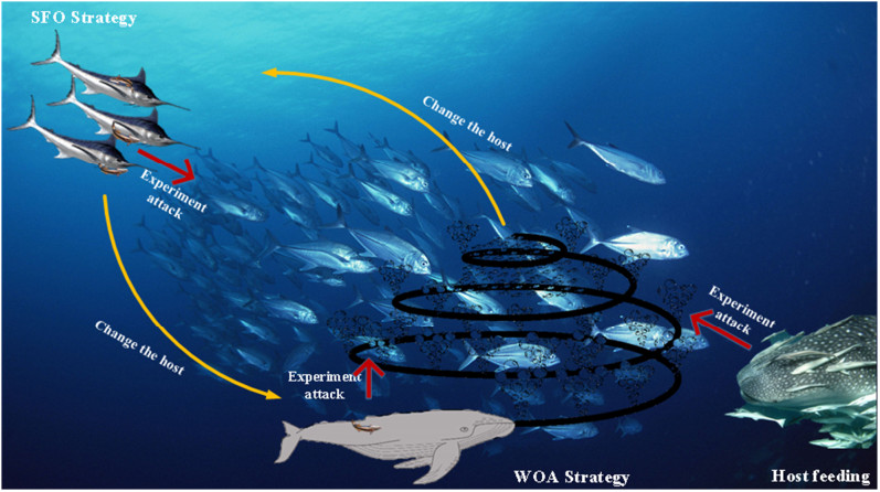
The remora optimization algorithm (ROA) is a newly proposed metaheuristic algorithm for solving global optimization problems. In ROA, each search agent searches new space according to the position of host, which makes the algorithm suffer from the drawbacks of slow convergence rate, poor solution accuracy, and local optima for some optimization problems. To tackle these problems, this study proposes an improved ROA (IROA) by introducing a new mechanism named autonomous foraging mechanism (AFM), which is inspired from the fact that remora can also find food on its own. In AFM, each remora has a small chance to search food randomly or according to the current food position. Thus the AFM can effectively expand the search space and improve the accuracy of the solution. To substantiate the efficacy of the proposed IROA, twenty-three classical benchmark functions and ten latest CEC 2021 test functions with various types and dimensions were employed to test the performance of IROA. Compared with seven metaheuristic and six modified algorithms, the results of test functions show that the IROA has superior performance in solving these optimization problems. Moreover, the results of five representative engineering design optimization problems also reveal that the IROA has the capability to obtain the optimal results for real-world optimization problems. To sum up, these test results confirm the effectiveness of the proposed mechanism.

| [1] |
K. Hussain, M. N. Mohd Salleh, S. Cheng, Y. Shi, Metaheuristic research: a comprehensive survey, Artif. Intell. Rev., 52 (2019), 2191-2233. https://doi.org/10.1007/s10462-017-9605-z doi: 10.1007/s10462-017-9605-z

|
| [2] |
W. Qiao, H. Moayedi, L. K. Foong, Nature-inspired hybrid techniques of IWO, DA, ES, GA, and ICA, validated through a k-fold validation process predicting monthly natural gas consumption, Energy Build., 217 (2020), 110023. https://doi.org/10.1016/j.enbuild.2020.110023 doi: 10.1016/j.enbuild.2020.110023
|
| [3] |
M. Wang, H. Chen, Chaotic multi-swarm whale optimizer boosted support vector machine for medical diagnosis, Appl. Soft Comput., 88 (2020), 105946. https://doi.org/10.1016/j.asoc.2019.105946 doi: 10.1016/j.asoc.2019.105946
|
| [4] |
S. Wang, J. Xiang, Y. Zhong, Y. Zhou, Convolutional neural network-based hidden Markov models for rolling element bearing fault identification, Knowl.-Based Syst., 144 (2018), 65-76. https://doi.org/10.1016/j.knosys.2017.12.027 doi: 10.1016/j.knosys.2017.12.027
|
| [5] |
H. Chen, Y. Xu, M. Wang, X. Zhao, A balanced whale optimization algorithm for constrained engineering design problems, Appl. Math. Model., 71 (2019), 45-59. https://doi.org/10.1016/j.apm.2019.02.004 doi: 10.1016/j.apm.2019.02.004
|
| [6] | J. Kennedy, R. Eberhart, Particle swarm optimization, in Proceedings of ICNN'95 - International Conference on Neural Networks, 4 (1995), 1942-1948. https://doi.org/10.1109/ICNN.1995.488968 |
| [7] | S. Mirjalili, A. Lewis, The whale optimization algorithm, Adv. Eng. Software, 95 (2016), 51-67. https://doi.org/10.1016/j.advengsoft.2016.01.008 |
| [8] | S. Mirjalili, S. M. Mirjalili, A. Lewis, Grey wolf optimizer, Adv. Eng. Software, 69 (2014), 46-61. https://doi.org/10.1016/j.advengsoft.2013.12.007 |
| [9] | G. Wang, S. Deb, Z. Cui, Monarch butterfly optimization, Neural Comput. Appl., 31 (2019), 1995-2014. https://doi.org/10.1007/s00521-015-1923-y |
| [10] | L. Abualigah, A. Diabat, S. Mirjalili, M. A. Elaziz, A. H. Gandomi, The arithmetic optimization algorithm, Comput. Methods Appl. Mech. Eng., 376 (2021), 113609. https://doi.org/10.1016/j.cma.2020.113609 |
| [11] |
S. Li, H. Chen, M. Wang, A. A. Heidari, S. Mirjalili, Slime mould algorithm: a new method for stochastic optimization, Future Gener. Comput. Syst., 111 (2020), 300-323. https://doi.org/10.1016/j.future.2020.03.055 doi: 10.1016/j.future.2020.03.055
|
| [12] | S. Mirjalili, The ant lion optimizer, Adv. Eng. Software, 83 (2015), 80-98. https://doi.org/10.1016/j.advengsoft.2015.01.010 |
| [13] |
S. Mirjalili, A. H. Gandomi, S. Z. Mirjalili, S. Saremi, H. Faris, S. M. Mirjalili, Salp swarm algorithm: a bio-inspired optimizer for engineering design problems, Adv. Eng. Software, 114 (2017), 163-191. https://doi.org/10.1016/j.advengsoft.2017.07.002 doi: 10.1016/j.advengsoft.2017.07.002
|
| [14] |
S. Saremi, S. Mirjalili, A. Lewis, Grasshopper optimization algorithm: theory and application, Adv. Eng. Software, 105 (2017), 30-47. https://doi.org/10.1016/j.advengsoft.2017.01.004 doi: 10.1016/j.advengsoft.2017.01.004
|
| [15] |
A. A. Heidari, S. Mirjalili, H. Faris, I. Aljarah, M. Mafarja, H. Chen, Harris hawks optimization: algorithm and applications, Future Gener. Comput. Syst., 97 (2019), 849-872. https://doi.org/10.1016/j.future.2019.02.028 doi: 10.1016/j.future.2019.02.028
|
| [16] |
A. Faramarzi, M. Heidarinejad, S. Mirjalili, A. H. Gandomi, Marine predators algorithm: a nature-inspired metaheuristic, Expert Syst. Appl., 152 (2020), 113377. https://doi.org/10.1016/j.eswa.2020.113377 doi: 10.1016/j.eswa.2020.113377
|
| [17] |
L. Abualigah, D. Yousri, M. A. Elaziz, A. A. Ewees, M. A. A. Al-qaness, A. H. Gandomi, Aquila optimizer: a novel meta-heuristic optimization algorithm, Comput. Ind. Eng., 157 (2021), 107250. https://doi.org/10.1016/j.cie.2021.107250 doi: 10.1016/j.cie.2021.107250
|
| [18] |
B. Abdollahzadeh, F. S. Gharehchopogh, S. Mirjalili, Artificial gorilla troops optimizer: a new nature-inspired metaheuristic algorithm for global optimization problems, Int. J. Intell. Syst., 36 (2021), 5887-5958. https://doi.org/10.1002/int.22535 doi: 10.1002/int.22535
|
| [19] |
B. Abdollahzadeh, F. S. Gharehchopogh, S. Mirjalili, African vultures optimization algorithm: a new nature-inspired metaheuristic algorithm for global optimization problems, Comput. Ind. Eng., 158 (2021), 107408. https://doi.org/10.1016/j.cie.2021.107408 doi: 10.1016/j.cie.2021.107408
|
| [20] |
I. Naruei, F. Keynia, Wild horse optimizer: a new meta-heuristic algorithm for solving engineering optimization problems, Eng. Comput., 2021. https://doi.org/10.1007/s00366-021-01438-z doi: 10.1007/s00366-021-01438-z
|
| [21] | Y. Yang, H. Chen, A. A. Heidari, A. H. Gandomi, Hunger games search: visions, conception, implementation, deep analysis, perspectives, and towards performance shifts, Expert Syst. Appl., 177 (2021), 114864. https://doi.org/10.1016/j.eswa.2021.114864 |
| [22] | J. Tu, H. Chen, M. Wang, A. H. Gandomi, The colony predation algorithm, J. Bionic Eng., 18 (2021), 674-710. https://doi.org/10.1007/s42235-021-0050-y |
| [23] |
D. H. Wolpert, W. G. Macready, No free lunch theorems for optimization, IEEE Trans. Evol. Comput., 1 (1997), 67-82. https://doi.org/10.1109/4235.585893 doi: 10.1109/4235.585893
|
| [24] |
M. A. A. Al-qaness, A. A. Ewees, M. A. Elaziz, Modified whale optimization algorithm for solving unrelated parallel machine scheduling problems, Soft Comput., 25 (2021), 9545-9557. https://doi.org/10.1007/s00500-021-05889-w doi: 10.1007/s00500-021-05889-w
|
| [25] |
A. A. Ewees, M. A.A. Al-qaness, M. A. Elaziz, Enhanced salp swarm algorithm based on firefly algorithm for unrelated parallel machine scheduling with setup times, Appl. Math. Model., 94 (2021), 285-305. https://doi.org/10.1016/j.apm.2021.01.017 doi: 10.1016/j.apm.2021.01.017
|
| [26] |
F. K. Onay, S. B. Aydemir, Chaotic hunger games search optimization algorithm for global optimization and engineering problems, Math. Comput. Simul., 192 (2021), 514-536. https://doi.org/10.1016/j.matcom.2021.09.014 doi: 10.1016/j.matcom.2021.09.014
|
| [27] | H. Jia, X. Peng, C. Lang, Remora optimization algorithm, Expert Syst. Appl., 185 (2021), 115665. https://doi.org/10.1016/j.eswa.2021.115665 |
| [28] |
S. Shadravan, H. R. Naji, V. K. Bardsiri, The sailfish optimizer: a novel nature-inspired metaheuristic algorithm for solving constrained engineering optimization problems, Eng. Appl. Artif. Intell., 80 (2019), 20-34. https://doi.org/10.1016/j.engappai.2019.01.001 doi: 10.1016/j.engappai.2019.01.001
|
| [29] |
A. A. Heidari, P. Pahlavani, An efficient modified grey wolf optimizer with Lévy Flight for Optimization Tasks, Appl. Soft Comput., 60 (2017), 115-134. https://doi.org/10.1016/j.asoc.2017.06.044 doi: 10.1016/j.asoc.2017.06.044
|
| [30] | M. Molga, C. Smutnicki, Test functions for optimization needs, 2005. |
| [31] |
R. Zheng, H. Jia, L. Abualigah, Q. Liu, S. Wang, Deep ensemble of slime mold algorithm and arithmetic optimization algorithm for global optimization, Process, 9 (2021), 1774. https://doi.org/10.3390/pr9101774 doi: 10.3390/pr9101774
|
| [32] |
L. Abualigah, M. A. Elaziz, P. Sumari, Z. W. Geem, A. H. Gandomi, Reptile Search Algorithm (RSA): a nature-inspired meta-heuristic optimizer, Expert Syst. Appl., 191 (2022), 116158. https://doi.org/10.1016/j.eswa.2021.116158 doi: 10.1016/j.eswa.2021.116158
|
| [33] |
E. H. Houssein, N. Neggaz, M. E. Hosney, W. M. Mohamed, M. Hassaballah, Enhanced Harris hawks optimization with genetic operators for selection chemical descriptors and compounds activities, Neural Comput. Appl., 33 (2021), 13601-13618. https://doi.org/10.1007/s00521-021-05991-y doi: 10.1007/s00521-021-05991-y
|
| [34] |
L. Rodríguez, O. Castillo, M. García, J. Soria, A new randomness approach based on sine waves to improve performance in metaheuristic algorithms, Soft. Comput., 24 (2020), 11989-12011. https://doi.org/10.1007/s00500-019-04641-9 doi: 10.1007/s00500-019-04641-9
|
| [35] |
W. Long, J. Jiao, X. Liang, S. Cai, M. Xu, A random opposition-based learning grey wolf optimizer, IEEE Access, 7 (2019), 113810-113825. https://doi.org/10.1109/ACCESS.2019.2934994 doi: 10.1109/ACCESS.2019.2934994
|
| [36] |
Y. Li, Y. Zhao, J. Liu, Dynamic sine cosine algorithm for large-scale global optimization problems, Expert Syst. Appl., 173 (2021), 114950. https://doi.org/10.1016/j.eswa.2021.114950 doi: 10.1016/j.eswa.2021.114950
|
| [37] |
S. Wang, K. Sun, W. Zhang, H. Jia, Multilevel thresholding using a modified ant lion optimizer with opposition-based learning for color image segmentation, Math. Biosci. Eng., 18 (2021), 3092-3143. https://doi.org/10.3934/mbe.2021155 doi: 10.3934/mbe.2021155
|
| [38] |
N. Singh, J. Kaur, Hybridizing sine-cosine algorithm with harmony search strategy for optimization design problems, Soft Comput., 25 (2021), 11053-11075. https://doi.org/10.1007/s00500-021-05841-y doi: 10.1007/s00500-021-05841-y
|
| [39] |
S. García, A. Fernández, J. Luengo, F. Herrera, Advanced nonparametric tests for multiple comparisons in the design of experiments in computational intelligence and data mining: experimental analysis of power, Inf. Sci., 180 (2010), 2044-2064. https://doi.org/10.1016/j.ins.2009.12.010 doi: 10.1016/j.ins.2009.12.010
|
| [40] |
E. Theodorsson-Norheim, Friedman and Quade tests: BASIC computer program to perform nonparametric two-way analysis of variance and multiple comparisons on ranks of several related samples, Comput. Biol. Med., 17 (1987), 85-99. https://doi.org/10.1016/0010-4825(87)90003-5 doi: 10.1016/0010-4825(87)90003-5
|
| [41] |
C. A. Coello, Use of a self-adaptive penalty approach for engineering optimization problems, Comput. Ind., 41 (2000), 113-127. https://doi.org/10.1016/S0166-3615(99)00046-9 doi: 10.1016/S0166-3615(99)00046-9
|
| [42] | E. Rashedi, H. Nezamabadi-pour, S. Saryazdi, GSA: a gravitational search algorithm, Inf. Sci., 179 (2009), 2232-2248. https://doi.org/10.1016/j.ins.2009.03.004 |
| [43] |
F. Huang, L. Wang, Q. He, An effective co-evolutionary differential evolution for constrained optimization, Appl. Math. Comput., 186 (2007), 340-356. https://doi.org/10.1016/j.amc.2006.07.105 doi: 10.1016/j.amc.2006.07.105
|
| [44] |
Q. He, L. Wang, An effective co-evolutionary particle swarm optimization for constrained engineering design problems, Eng. Appl. Artif. Intell., 20 (2007), 89-99. https://doi.org/10.1016/j.engappai.2006.03.003 doi: 10.1016/j.engappai.2006.03.003
|
| [45] |
A. Baykasoğlu, S. Akpinar, Weighted superposition attraction (WSA): A swarm intelligence algorithm for optimization problems-part2: Constrained optimization, Appl. Soft Comput., 37 (2015), 396-415. https://doi.org/10.1016/j.asoc.2015.08.052 doi: 10.1016/j.asoc.2015.08.052
|
| [46] |
H. Yapici, N. Cetinkaya, A new meta-heuristic optimizer: pathfinder algorithm, Appl. Soft Comput., 78 (2019), 545-568. https://doi.org/10.1016/j.asoc.2019.03.012 doi: 10.1016/j.asoc.2019.03.012
|
| [47] | Q. Fan, H. Huang, Q. Chen, L. Yao, K. Yang, D. Huang, A modified self-adaptive marine predators algorithm: framework and engineering applications, Eng. Comput., (2021). https://doi.org/10.1007/s00366-021-01319-5 |
| [48] |
W. Long, T. Wu, X. Liang, S. Xu, Solving high-dimensional global optimization problems using an improved sine cosine algorithm, Expert Syst. Appl., 123 (2019), 108-126. https://doi.org/10.1016/j.eswa.2018.11.032 doi: 10.1016/j.eswa.2018.11.032
|
| [49] |
Y. Li, X. Zhu, J. Liu, An improved moth-flame optimization algorithm for engineering problems, Symmetry, 12 (2020), 1234. https://doi.org/10.3390/sym12081234 doi: 10.3390/sym12081234
|
| [50] |
T. Ray, P. Saini, Engineering design optimization using a swarm with an intelligent information sharing among individuals, Eng. Optim., 33 (2001), 735-748. https://doi.org/10.1080/03052150108940941 doi: 10.1080/03052150108940941
|
| [51] |
S. Mirjalili, Moth-flame optimization algorithm: a novel nature-inspired heuristic paradigm, Knowl.-Based Syst., 89 (2015), 228-249. https://doi.org/10.1016/j.knosys.2015.07.006 doi: 10.1016/j.knosys.2015.07.006
|
| [52] |
H. Liu, Z. Cai, Y. Wang, Hybridizing particle swarm optimization with differential evolution for constrained numerical and engineering optimization, Appl. Soft Comput., 10 (2010), 629-640. https://doi.org/10.1016/j.asoc.2009.08.031 doi: 10.1016/j.asoc.2009.08.031
|
| [53] |
L. Gu, R. J. Yang, C. H. Tho, M. Makowskit, O. Faruquet, Y. Li, Optimisation and robustness for crashworthiness of side impact, Int. J. Veh. Des., 26 (2001), 348-360. https://doi.org/10.1504/IJVD.2001.005210 doi: 10.1504/IJVD.2001.005210
|
| [54] |
B. S. Yildiz, N. Pholdee, S. Bureerat, A. R. Yildiz, S. M. Sait, Enhanced grasshopper optimization algorithm using elite opposition-based learning for solving real-world engineering problems, Eng. Comput., 2021. https://doi.org/10.1007/s00366-021-01368-w doi: 10.1007/s00366-021-01368-w
|
| [55] | S. S. Rao, Engineering optimization: Theory and Practice, 3rd edn. John Wiley & Sons, Chichester, 1996. |
| [56] |
A. H. Gandomi, X. S. Yang, A. H. Alavi, Cuckoo search algorithm: a metaheuristic approach to solve structural optimization problems, Eng. Comput., 29 (2013), 17-35. https://doi.org/10.1007/s00366-011-0241-y doi: 10.1007/s00366-011-0241-y
|


Figures(12) / Tables(15)

Rong Zheng, Heming Jia, Laith Abualigah, Shuang Wang, Di Wu. An improved remora optimization algorithm with autonomous foraging mechanism for global optimization problems[J]. Mathematical Biosciences and Engineering, 2022, 19(4): 3994-4037. doi: 10.3934/mbe.2022184


 DownLoad: