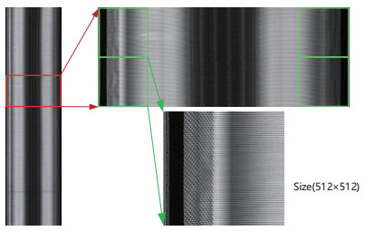
The tire factory mainly inspects tire quality through X-ray images. In this paper, an end-to-end lightweight semantic segmentation network is proposed to realize the error detection of bead toe. In the network, firstly, the texture feature of different regions of tire is extracted by an encoder. Then, we introduce a decoder to fuse the output feature of the encoder. As the dimension of the feature maps is reduced, the positions of bead toe in the X-ray image have been recorded. When evaluating the final segmentation effect, we propose a local mIoU(L-mIoU) index. The segmentation accuracy and reasoning speed of the network are verified on the tire X-ray image set. Specifically, for 512 $ \times $ 512 input images, we achieve 97.1% mIoU and 92.4% L-mIoU. Alternatively, the bead toe coordinates are calculated using only 1.0 s.
Citation: Xin Yi, Chen Peng, Zhen Zhang, Liang Xiao. The defect detection for X-ray images based on a new lightweight semantic segmentation network[J]. Mathematical Biosciences and Engineering, 2022, 19(4): 4178-4195. doi: 10.3934/mbe.2022193
The tire factory mainly inspects tire quality through X-ray images. In this paper, an end-to-end lightweight semantic segmentation network is proposed to realize the error detection of bead toe. In the network, firstly, the texture feature of different regions of tire is extracted by an encoder. Then, we introduce a decoder to fuse the output feature of the encoder. As the dimension of the feature maps is reduced, the positions of bead toe in the X-ray image have been recorded. When evaluating the final segmentation effect, we propose a local mIoU(L-mIoU) index. The segmentation accuracy and reasoning speed of the network are verified on the tire X-ray image set. Specifically, for 512 $ \times $ 512 input images, we achieve 97.1% mIoU and 92.4% L-mIoU. Alternatively, the bead toe coordinates are calculated using only 1.0 s.

| [1] | Centers for Disease Control and Prevention, Leading Causes of Death, National Center for Health Statistics, 2020. Available from: https://www.cdc.gov/nchs/fastats/leading-causes-of-death.htm. |
| [2] | National Highway Traffic Safety Administration, Safety and Savings Ride on Your Tires, Always Perform Proper Maintenance, 2020. Available from: https://www.nhtsa.gov/es/tires/safety-and-savings-ride-your-tires. |
| [3] |
L. Sun, L. He, C. Hai, X. Han, Z. Gui, M. Yang, Design of imaging system and tomography detection method for radial tires structure under X-ray short-scan mode, IEEE Trans. Instrum. Meas., 70 (2021), 1–12. https://doi.org/10.1109/TIM.2021.3118098 doi: 10.1109/TIM.2021.3118098

|
| [4] |
G. Fortunato, V. Ciaravola, A. Furno, M. Scaraggi, B. Lorenz, B. N. Persson, Dependency of rubber friction on normal force or load: theory and experiment, Tire Sci. Technol., 45 (2017), 25–54. https://doi.org/10.2346/tire.17.450103 doi: 10.2346/tire.17.450103
|
| [5] |
J. J. Castillo Aguilar, J. A. C. Carrillo, A. J. G. Fernández, S. P. Pozo, Optimization of an optical test bench for tire properties measurement and tread defects characterization, Tire Sci. Technol., 17 (2017), 707. https://doi.org/10.3390/s17040707 doi: 10.3390/s17040707
|
| [6] |
X. Cui, Y. Liu, Y. Zhang, C. Wang, Tire defects classification with multi-contrast convolutional neural networks, Int. J. Pattern Recogn., 32 (2018), 1850011. https://doi.org/10.1142/S0218001418500118 doi: 10.1142/S0218001418500118
|
| [7] |
Q. Guo, C. Zhang, H. Liu, X. Zhang, Defect detection in tire X-ray images using weighted texture dissimilarity, J. Sens., 32 (2016), 2016. https://doi.org/10.1155/2016/4140175 doi: 10.1155/2016/4140175
|
| [8] |
Y. Zhang, T. Li, Q. Li, Detection of foreign bodies and bubble defects in tire radiography images based on total variation and edge detection, Chin. Phys. Lett., 30 (2013), 084205. https://doi.org/10.1088/0256-307X/30/8/084205 doi: 10.1088/0256-307X/30/8/084205
|
| [9] |
Y. Zhang, T. Li, Q. Li, Defect detection for tire laser shearography image using curvelet transform based edge detector, Opt. Laser Technol., 47 (2013), 64–71. https://doi.org/10.1016/j.optlastec.2012.08.023 doi: 10.1016/j.optlastec.2012.08.023
|
| [10] |
Y. Zhang, D. Lefebvre, Q. Li, Automatic detection of defects in tire radiographic images, IEEE Trans. Autom. Sci. Eng., 14 (2015), 1378–1386. https://doi.org/10.1109/TASE.2015.2469594 doi: 10.1109/TASE.2015.2469594
|
| [11] |
G. Zhao, S. Qin, High-precision detection of defects of tire texture through X-ray imaging based on local inverse difference moment features, Sensors, 18 (2018), 2524. https://doi.org/10.3390/s18082524 doi: 10.3390/s18082524
|
| [12] |
S. Jia, S. Jiang, Z. Lin, N. Li, M. Xu, S. Yu, A survey: Deep learning for hyperspectral image classification with few labeled samples, Neurocomputing, 448 (2021), 179–204. https://doi.org/10.1016/j.neucom.2021.03.035 doi: 10.1016/j.neucom.2021.03.035
|
| [13] |
K. Lan, G. Li, Y. Jie, R. Tang, L. Liu, S. Fong, Convolutional neural network with group theory and random selection particle swarm optimizer for enhancing cancer image classification, Math. Biosci. Eng., 18 (2021), 5573–5591. https://doi.org/10.3934/mbe.2021281 doi: 10.3934/mbe.2021281
|
| [14] |
Y. Liu, P. Sun, N. Wergeles, Y. Shang, A survey and performance evaluation of deep learning methods for small object detection, Expert Syst. Appl., 172 (2021), 114602. https://doi.org/10.1016/j.eswa.2021.114602 doi: 10.1016/j.eswa.2021.114602
|
| [15] |
H. Ni, M. Wang, L. Zhao, An improved Faster R-CNN for defect recognition of key components of transmission line, Math. Biosci. Eng., 18 (2021), 4679–4695. https://doi.org/10.3934/mbe.2021237 doi: 10.3934/mbe.2021237
|
| [16] |
Q. Zhou, X. Wu, S. Zhang, B. Kang, Z. Ge, L. J. Latecki, Contextual ensemble network for semantic segmentation, Pattern Recognit., 122 (2022), 108290. https://doi.org/10.1016/j.patcog.2021.108290 doi: 10.1016/j.patcog.2021.108290
|
| [17] |
W. Lu, J. Chen, F. Xue, Using computer vision to recognize composition of construction waste mixtures: A semantic segmentation approach, Resour. Conserv. Recycl., 178 (2022), 106022. https://doi.org/10.1016/j.resconrec.2021.106022 doi: 10.1016/j.resconrec.2021.106022
|
| [18] |
R. Ren, T. Hung, K. C. Tan, A generic deep-learning-based approach for automated surface inspection, IEEE Trans. Cybern., 48 (2018), 929–940. https://doi.org/10.1109/TCYB.2017.2668395 doi: 10.1109/TCYB.2017.2668395
|
| [19] |
W. Lu, J. Chen, F. Xue, Using computer vision to recognize composition of construction waste mixtures: A semantic segmentation approach, Resour. Conserv. Recycl., 178 (2022), 106022. https://doi.org/10.1016/j.resconrec.2021.106022 doi: 10.1016/j.resconrec.2021.106022
|
| [20] | K. He, X. Zhang, S. Ren, J. Su, Deep residual learning for image recognition, in Proceedings of the IEEE Conference on Computer Vision and Pattern Recognition, IEEE, (2016), 770–778. https://doi.org/10.1109/cvpr.2016.90 |
| [21] |
L. Yang, H. Wang, B. Huo, F. Li, Y. Liu, An automatic welding defect location algorithm based on deep learning, NDT E Int., 120 (2021), 102435. https://doi.org/10.1016/j.ndteint.2021.102435 doi: 10.1016/j.ndteint.2021.102435
|
| [22] |
Y. Li, B. Fan, W. Zhang, Z. Jiang, TireNet: A high recall rate method for practical application of tire defect type classification, Future Gener. Comput. Syst., 125 (2021), 1–9. https://doi.org/10.1016/j.future.2021.06.009 doi: 10.1016/j.future.2021.06.009
|
| [23] |
Y. Zhang, X. Cui, Y. Liu, B. Yu, Tire defects classification using convolution architecture for fast feature embedding, Int. J. Comput., 11 (2018), 1056–1066. https://doi.org/10.2991/ijcis.11.1.80 doi: 10.2991/ijcis.11.1.80
|
| [24] | J. Long, E. Shelhamer, T. Darrell, Fully convolutional networks for semantic segmentation, in IEEE Conference on Computer Vision and Pattern Recognition, IEEE, (2015), 3431-3440. https://doi.org/10.1109/cvpr.2015.7298965 |
| [25] | O. Ronneberger, P. Fischer, T. Brox, U-net: Convolutional networks for biomedical image segmentation, in International Conference on Medical Image Computing and Computer-Assisted Intervention, Springer, (2015), 234-241. https://doi.org/10.1007/978-3-319-24574-4_28 |
| [26] |
V. Badrinarayanan, A. Kendall, R. Cipolla, Segnet: A deep convolutional encoder-decoder architecture for image segmentation, IEEE Trans. Pattern Anal. Mach. Intell., 39 (2017), 2481–2495. https://doi.org/10.1109/tpami.2016.2644615 doi: 10.1109/tpami.2016.2644615
|
| [27] | C. Peng, X. Zhang, G. Yu, G. Luo, J. Sun, Large kernel matters–improve semantic segmentation by global convolutional network, in IEEE Conference on Computer Vision and Pattern Recognition, IEEE, (2017), 4353-4361. https://doi.org/10.1109/CVPR.2017.189 |
| [28] | G. GhiasiEmail, C. C. Fowlkes, Laplacian pyramid reconstruction and refinement for semantic segmentation, in European Conference on Computer Vision, Springer, (2017), 519-534. https://doi.org/10.1007/978-3-319-46487-9_32 |
| [29] |
V. Badrinarayanan, A. Kendall, R. Cipolla, A nonlocal deep image prior model to restore optical coherence tomographic images from gamma distributed speckle noise, J. Mod. Opt., 68 (2021), 1002–1017. https://doi.org/10.1080/09500340.2021.1968052 doi: 10.1080/09500340.2021.1968052
|
| [30] | A. Paszke, A. Chaurasia, S. Kim, E. Culurciello, Enet: A deep neural network architecture for real-time semantic segmentation, preprint, arXiv: 1606.02147. |
| [31] | C. Yu, J. Wang, C. Peng, C. Gao, G. Yu, N. Sang, Bisenet: Bilateral segmentation network for real-time semantic segmentation, in European Conference on Computer Vision, Springer, (2018), 325–341. https://doi.org/10.1007/978-3-030-01261-8_20 |
| [32] | M. Fan, S. Lai, J. Huang, X. Wei, Z. Chai, J. Luo, et al., Rethinking BiSeNet for real-time semantic segmentation, in IEEE Conference on Computer Vision and Pattern Recognition, IEEE, (2015), 9716–9725. https://doi.org/10.1109/cvpr46437.2021.00959 |
| [33] | V. Nekrasov, C. Shen, I. Reid, Light-weight refinenet for real-time semantic segmentation, preprint, arXiv: 1810.03272. |
| [34] | H. Si, Z. Zhang, F. Lv, G. Yu, F. Lu, Real-time semantic segmentation via multiple spatial fusion network, preprint, arXiv: 1911.07217. |


Figures(11) / Tables(5)

Xin Yi, Chen Peng, Zhen Zhang, Liang Xiao. The defect detection for X-ray images based on a new lightweight semantic segmentation network[J]. Mathematical Biosciences and Engineering, 2022, 19(4): 4178-4195. doi: 10.3934/mbe.2022193


 DownLoad: