Immuno-epidemiological co-affection model of HIV infection and opioid addiction

Churni Gupta; Necibe Tuncer; Maia Martcheva; Churni Gupta; Necibe Tuncer; Maia Martcheva

doi:10.3934/mbe.2022168

Mathematical Biosciences and Engineering

2022, Volume 19, Issue 4: 3636-3672. doi: 10.3934/mbe.2022168

Previous Article Next Article

Research article

Immuno-epidemiological co-affection model of HIV infection and opioid addiction

1.
Faculty of Pharmacy, University of Montreal, Montreal, QC, Canada
2.
Department of Mathematical Sciences, Florida Atlantic University, Boca Raton, FL, United States of America
3.
Department of Mathematics, University of Florida, Gainesville, FL, United States of America

Academic Editor: Amina Eladdadi

Received: 10 November 2021 Revised: 12 January 2022 Accepted: 17 January 2022 Published: 08 February 2022

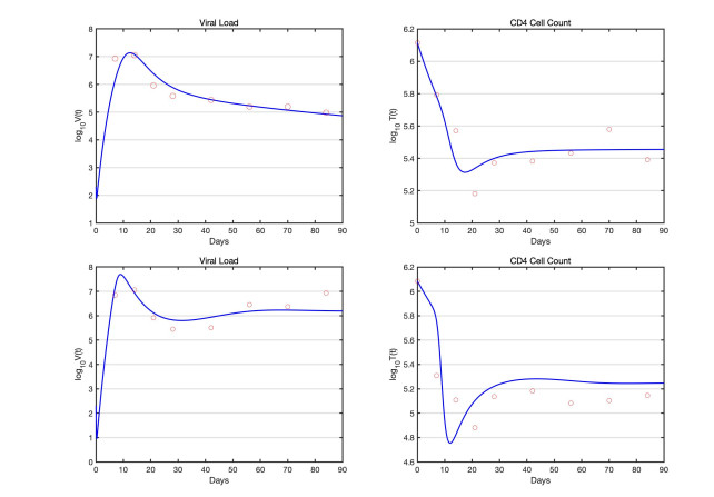
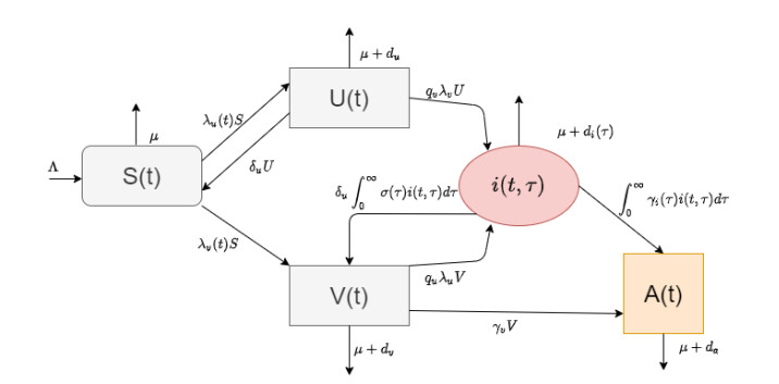
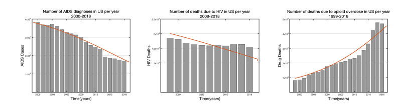
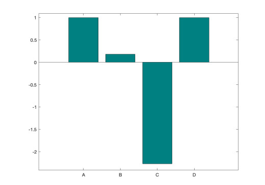
In this paper, we present a multi-scale co-affection model of HIV infection and opioid addiction. The population scale epidemiological model is linked to the within-host model which describes the HIV and opioid dynamics in a co-affected individual. CD4 cells and viral load data obtained from morphine addicted SIV-infected monkeys are used to validate the within-host model. AIDS diagnoses, HIV death and opioid mortality data are used to fit the between-host model. When the rates of viral clearance and morphine uptake are fixed, the within-host model is structurally identifiable. If in addition the morphine saturation and clearance rates are also fixed the model becomes practical identifiable. Analytical results of the multi-scale model suggest that in addition to the disease-addiction-free equilibrium, there is a unique HIV-only and opioid-only equilibrium. Each of the boundary equilibria is stable if the invasion number of the other epidemic is below one. Elasticity analysis suggests that the most sensitive number is the invasion number of opioid epidemic with respect to the parameter of enhancement of HIV infection of opioid-affected individual. We conclude that the most effective control strategy is to prevent opioid addicted individuals from getting HIV, and to treat the opioid addiction directly and independently from HIV.
- co-affection,
- multi-scale,
- HIV,
- opioid addiction,
- elasticity analysis,
- identifiable,
- invasion numbers,
- data fitting,
- immuno-epidemiological model
Citation: Churni Gupta, Necibe Tuncer, Maia Martcheva. Immuno-epidemiological co-affection model of HIV infection and opioid addiction[J]. Mathematical Biosciences and Engineering, 2022, 19(4): 3636-3672. doi: 10.3934/mbe.2022168

Related Papers:

Abstract

In this paper, we present a multi-scale co-affection model of HIV infection and opioid addiction. The population scale epidemiological model is linked to the within-host model which describes the HIV and opioid dynamics in a co-affected individual. CD4 cells and viral load data obtained from morphine addicted SIV-infected monkeys are used to validate the within-host model. AIDS diagnoses, HIV death and opioid mortality data are used to fit the between-host model. When the rates of viral clearance and morphine uptake are fixed, the within-host model is structurally identifiable. If in addition the morphine saturation and clearance rates are also fixed the model becomes practical identifiable. Analytical results of the multi-scale model suggest that in addition to the disease-addiction-free equilibrium, there is a unique HIV-only and opioid-only equilibrium. Each of the boundary equilibria is stable if the invasion number of the other epidemic is below one. Elasticity analysis suggests that the most sensitive number is the invasion number of opioid epidemic with respect to the parameter of enhancement of HIV infection of opioid-affected individual. We conclude that the most effective control strategy is to prevent opioid addicted individuals from getting HIV, and to treat the opioid addiction directly and independently from HIV.

References

[1]	World Health Organization, HIV/AIDS, Available from: https://www.who.int/data/gho/data/themes/hiv-aids.
[2]	N. Dorratoltaj, R. Nikin-Beers, S. M. Ciupe, S. G. Eubank, K. M. Abbas, Multi-scale immunoepidemiological modeling of within-host and between-host HIV dynamics: systematic review of mathematical models, PeerJ, 5 (2017), e3877. https://doi.org/10.7717/peerj.3877 doi: 10.7717/peerj.3877
[3]	M. Martcheva, X. Z. Li, Linking immunological and epidemiological dynamics of HIV: the case of super-infection, J. Biol. Dyn., 7 (2013), 161–182. https://doi.org/10.1080/17513758.2013.820358 doi: 10.1080/17513758.2013.820358
[4]	A. S. Perelson, P. W. Nelson, Mathematical analysis of HIV-1: Dynamics in vivo, SIAM Rev., 41 (1999), 3–44. https://doi.org/10.1137/S0036144598335107 doi: 10.1137/S0036144598335107
[5]	M. Shen, Y. Xiao, L. Rong, L. A. Meyers, Conflict and accord of optimal treatment strategies for HIV infection within and between hosts, Math. Biosci., 309 (2019), 107–117. https://doi.org/10.1016/j.mbs.2019.01.007 doi: 10.1016/j.mbs.2019.01.007
[6]	R. Rothenberg, HIV transmission networks, Curr. Opin. HIV AIDS, 4 (2009), 260–265. https://doi.org/10.1097/COH.0b013e32832c7cfc doi: 10.1097/COH.0b013e32832c7cfc
[7]	National Institute of Drug Abuse (NIH), Opioid overdose crisis. Available from: https://www.drugabuse.gov/drug-topics/opioids/opioid-overdose-crisis.
[8]	S. L. Hodder, J. Feinberg, S. A. Strathdee, S. Shoptaw, F. L. Altice, L. Ortenzio, et al., The opioid crisis and HIV in the USA: deadly synergies, Lancet, 397 (2021), 1139–1150, https://doi.org/10.1016/S0140-6736(21)00391-3 doi: 10.1016/S0140-6736(21)00391-3
[9]	P. Hughes, G. Crawford, A contagious disease model for researching and intervening in heroin epidemics, Arch. Gen. Psychiatry, 27 (1972), 149–155. https://doi.org/10.1001/archpsyc.1972.01750260005001 doi: 10.1001/archpsyc.1972.01750260005001
[10]	D. R. Mackintosh, G. T. Stewart, A mathematical model of a heroin epidemic: implications for control policies, J. Epidemiol. Community Health, 33 (1979), 299–304. https://doi.org/10.1136/jech.33.4.299 doi: 10.1136/jech.33.4.299
[11]	N. A. Battista, L. B. Pearcy, W. C. Strickland, Modeling the prescription opioid epidemic, Bull. Math. Biol., 81 (2019), 2258–2289. https://doi.org/10.1007/s11538-019-00605-0 doi: 10.1007/s11538-019-00605-0
[12]	S. Wakeman, T. Green, J. Rich, From documenting death to comprehensive care: Applying lessons from the HIV/AIDS epidemic to addiction, Am. J. Med., 127 (2014), 465–466. https://doi.org/10.1016/j.amjmed.2013.12.018 doi: 10.1016/j.amjmed.2013.12.018
[13]	A. Lemons, N. P. DeGroote, A. Pérez, J. A. Craw, M. Nyaku, D. Broz, et al., Opioid misuse among HIV-positive adults in medical care: Results from the medical monitoring project, 2009–2014, J. Acquir. Immune Defic. Syndr., 80 (2019), 127–134. https://doi.org/10.1097/QAI.0000000000001889 doi: 10.1097/QAI.0000000000001889
[14]	E. J. Edelman, K. S. Gordon, K. Crothers, K. Akgün, K. J. Bryant, W. C. Becker, et al., Association of prescribed opioids with increased risk of community-acquired pneumonia among patients with and without HIV, JAMA Intern. Med., 179 (2019), 297–304. https://doi.org/10.1001/jamainternmed.2018.6101 doi: 10.1001/jamainternmed.2018.6101
[15]	A. Murphy, J. Barbaro, P. Martínez-Aguado, V. Chilunda, M. Jaureguiberry-Bravo, J. W. Berman, The effects of opioids on HIV neuropathogenesis, Front. Immunol., 10 (2019), 2445. https://doi.org/10.3389/fimmu.2019.02445 doi: 10.3389/fimmu.2019.02445
[16]	Substance Use and HIV Risk. Available from: https://www.hiv.gov/hiv-basics/hiv-prevention/reducing-risk-from-alcohol-and-drug-use/substance-use-and-hiv-risk.
[17]	L. Fanucchi, S. Springer, T. Korthuis, Medications for treatment of opioid use disorder among persons living with HIV, Curr. HIV/AIDS Rep., 16 (2019), 1–6. https://doi.org/10.1007/s11904-019-00436-7 doi: 10.1007/s11904-019-00436-7
[18]	X. C. Duan, X. Z. Li, M. Martcheva, Coinfection dynamics of heroin transmission and HIV infection in a single population, J. Biol. Dyn., 14 (2020), 116–142. https://doi.org/10.1080/17513758.2020.1726516 doi: 10.1080/17513758.2020.1726516
[19]	M. Martcheva, An Introduction to Mathematical Epidemiology, Springer, New York, 2015. https://doi.org/10.1007/978-1-4899-7612-3_8
[20]	M. Gilchrist, A. Sasaki, Modeling host-parasite coevolution: a nested approach based on mechanistic models, J. Theor. Biol., 218 (2002), 289–308. https://doi.org/10.1006/jtbi.2002.3076 doi: 10.1006/jtbi.2002.3076
[21]	M. Nowak, R. May, Virus Dynamics: Mathematical Principles of Immunology and Virology, Oxford University Press, New York, USA, 2000.
[22]	N. K. Vaidya, R. M. Ribeiro, A. S. Perelson, A. Kumar, Modeling the effects of morphine on simian immunodeficiency virus dynamics, PLoS Comput. Biol., 19 (2016), e1005127. https://doi.org/10.1371/journal.pcbi.1005127 doi: 10.1371/journal.pcbi.1005127
[23]	R. Kumar, C. Torres, Y. Yamamura, I. Rodriguez, M. Martinez, S. Staprans, et al., Modulation by morphine of viral set point in rhesus macaques infected with simian immunodeficiency virus and simian-human immunodeficiency virus, J. Virol., 78 (2004), 11425–11428. https://doi.org/10.1128/JVI.78.20.11425-11428.2004 doi: 10.1128/JVI.78.20.11425-11428.2004
[24]	H. Miao, X. Xia, A. S. Perelson, H. Wu, On the identifiability of nonlinear ode models and applications in viral dynamics, SIAM Rev., 53 (2011), 3–39. https://doi.org/10.1137/090757009 doi: 10.1137/090757009
[25]	M. C. Eisenberg, S. L. Robertson, J. H. Tien, Identifiability and estimation of multiple transmission pathways in cholera and waterborne disease, J. Theor. Biol., 324 (2013), 84–102. https://doi.org/10.1016/j.jtbi.2012.12.021 doi: 10.1016/j.jtbi.2012.12.021
[26]	N. Tuncer, H. Gulbudak, V. L. Cannataro, M. Martcheva, Structural and practical identifiability issues of immuno-epidemiological vector-host models with application to Rift Valley Fever, Bull. Math. Biol., 78 (2016), 1796–1827. https://doi.org/10.1007/s11538-016-0200-2 doi: 10.1007/s11538-016-0200-2
[27]	N. Tuncer, M. Martcheva, B. Labarre, S. Payoute, Structural and practical identifiability analysis of Zika epidemiological models, Bull. Math. Biol., 80 (2018), 2209–2241. https://doi.org/10.1007/s11538-018-0453-z doi: 10.1007/s11538-018-0453-z
[28]	J. M. Mutua, A. S. Perelson, A. Kumar, N. Vaidya, Modeling the effects of morphine-altered virus-specific antibody responses on HIV/SIV dynamics, Sci. Rep., 9 (2019). https://doi.org/10.1038/s41598-019-41751-8
[29]	A. Lange, N. Ferguson, Antigenic diversity, transmission mechanisms, and the evolution of pathogens, PLoS Comput. Biol., 5 (2009), 12. https://doi.org/10.1371/journal.pcbi.1000536 doi: 10.1371/journal.pcbi.1000536
[30]	M. A. Gilchrist, D. Coombs, Evolution of virulence: Interdependence, constraints, and selection using nested models, Theor. Popul. Biol., 69 (2006), 145–153. https://doi.org/10.1016/j.tpb.2005.07.002 doi: 10.1016/j.tpb.2005.07.002
[31]	Centers for Disease Control and Prevention, Terms, definitions, and calculations used in CDC HIV surveillance publications. Available from: https://www.cdc.gov/hiv/pdf/statistics/systems/nhbs/cdc-hiv-terms-surveillance-publications-2014.pdf.
[32]	C. Gupta, N. Tuncer, M. Martcheva, A network immuno-epidemiological HIV model, Bull. Math. Biol., 83 (2020), 1–29. https://doi.org/10.1007/s11538-020-00855-3 doi: 10.1007/s11538-020-00855-3
[33]	J. S. Welker, M. Martcheva, Analysis and simulations with a multi-scale model of canine visceral leishmaniasis, Math. Model. Nat. Phenom., 15 (2020), 72–110. https://doi.org/10.1051/mmnp/2020026 doi: 10.1051/mmnp/2020026
[34]	N. Tuncer, S. Giri, Dynamics of a vector-borne model with direct transmission and age of infection, Math. Modell. Nat. Phenom., 16 (2021). https://doi.org/10.1051/mmnp/2021019
[35]	Centers for Disease Control and Prevention. Available from: https://www.cdc.gov/nchhstp/atlas/index.htm.
[36]	Drug overdose deaths in the united states, 1999–2018. Available from: https://www.cdc.gov/nchs/products/databriefs/db356.htm#ref1.
[37]	Drug overdose deaths in the united states, 1999–2018. Available from: https://www.cdc.gov/nchs/data/databriefs/db356_tables-508.pdf#page=1.

Reader Comments

Your name:*

Email:*
© 2022 the Author(s), licensee AIMS Press. This is an open access article distributed under the terms of the Creative Commons Attribution License (http://creativecommons.org/licenses/by/4.0)