Dynamics for a non-autonomous fall armyworm-maize interaction model with a saturation functional response

Salamida Daudi; Livingstone Luboobi; Moatlhodi Kgosimore; Dmitry Kuznetsov; Salamida Daudi; Livingstone Luboobi; Moatlhodi Kgosimore; Dmitry Kuznetsov

doi:10.3934/mbe.2022008

Mathematical Biosciences and Engineering

2022, Volume 19, Issue 1: 146-168. doi: 10.3934/mbe.2022008

Previous Article Next Article

Research article

Dynamics for a non-autonomous fall armyworm-maize interaction model with a saturation functional response

1.
School of Computational and Communication Science and Engineering, The Nelson Mandela African Institution of Science and Technology (NM-AIST), P. O. Box 447, Arusha, Tanzania
2.
Department of Mathematics, Humanities and Social Science (MHSS), National Institute of Transport (NIT), P.O. Box 705, Dar-es-Salaam, Tanzania
3.
Department of Mathematics, Makerere University, P.O. Box 7062, Kampala, Uganda
4.
Department of Biometry and Mathematics, Botswana University of Agriculture and Natural Resources, Private Bag 0027, Gaborone, Botswana

Academic Editor: Urszula Ledzewicz

Received: 14 July 2021 Accepted: 17 October 2021 Published: 09 November 2021

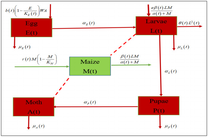
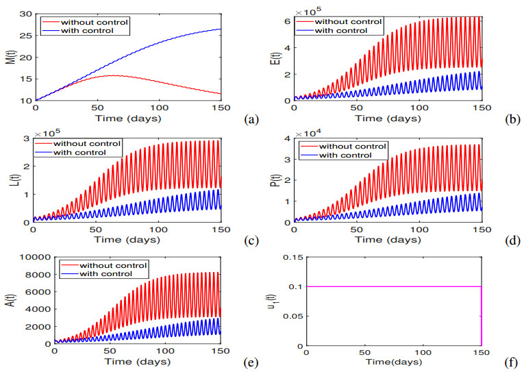
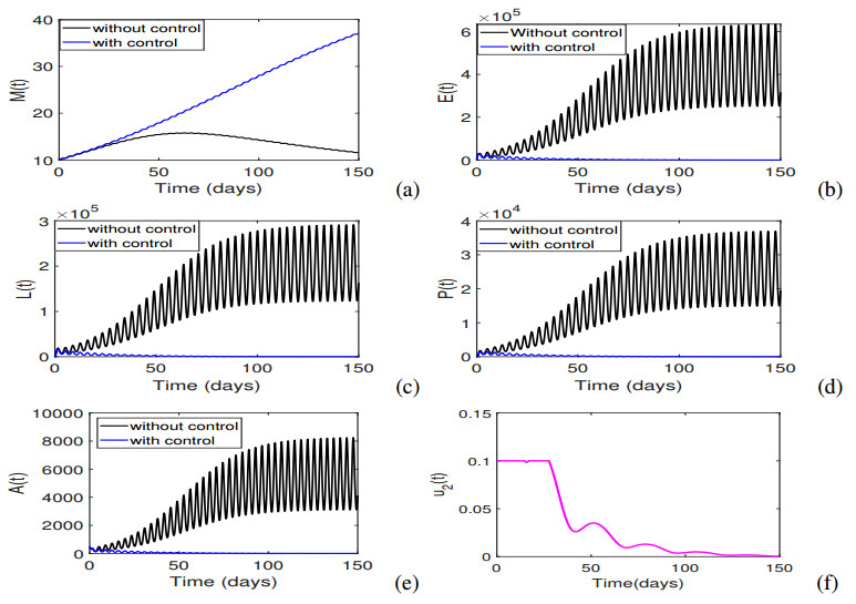
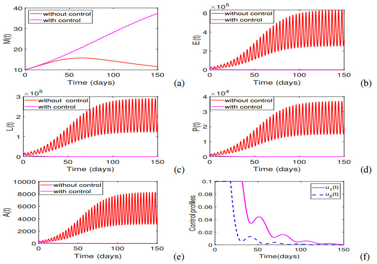
In this study, we present a non-autonomous model with a Holling type II functional response, to study the complex dynamics for fall armyworm-maize biomass interacting in a periodic environment. Understanding how seasonal variations affect fall armyworm-maize dynamics is critical since maize is one of the most important cereals globally. Firstly, we study the dynamical behaviours of the basic model; that is, we investigate positive invariance, boundedness, permanence, global stability and non-persistence. We then extended the model to incorporate time dependent controls. We investigate the impact of reducing fall armyworm egg and larvae population, at minimal cost, through traditional methods and use of chemical insecticides. We noted that seasonal variations play a significant role on the patterns for all fall armyworm populations (egg, larvae, pupae and moth). We also noted that in all scenarios, the optimal control can greatly reduce the sizes of fall armyworm populations and in some scenarios, total elimination may be attained. The modeling approach presented here provides a framework for designing effective control strategies to manage the fall armyworm during outbreaks.
- fall armyworm,
- maize,
- seasonal variations,
- mathematical model,
- optimal control
Citation: Salamida Daudi, Livingstone Luboobi, Moatlhodi Kgosimore, Dmitry Kuznetsov. Dynamics for a non-autonomous fall armyworm-maize interaction model with a saturation functional response[J]. Mathematical Biosciences and Engineering, 2022, 19(1): 146-168. doi: 10.3934/mbe.2022008

Related Papers:

Abstract

In this study, we present a non-autonomous model with a Holling type II functional response, to study the complex dynamics for fall armyworm-maize biomass interacting in a periodic environment. Understanding how seasonal variations affect fall armyworm-maize dynamics is critical since maize is one of the most important cereals globally. Firstly, we study the dynamical behaviours of the basic model; that is, we investigate positive invariance, boundedness, permanence, global stability and non-persistence. We then extended the model to incorporate time dependent controls. We investigate the impact of reducing fall armyworm egg and larvae population, at minimal cost, through traditional methods and use of chemical insecticides. We noted that seasonal variations play a significant role on the patterns for all fall armyworm populations (egg, larvae, pupae and moth). We also noted that in all scenarios, the optimal control can greatly reduce the sizes of fall armyworm populations and in some scenarios, total elimination may be attained. The modeling approach presented here provides a framework for designing effective control strategies to manage the fall armyworm during outbreaks.

References

[1]	S. Jeyaraman, Field Crops Production and Management, Oxford and IBH Publishing Company Pvt. Limited, 2017.
[2]	S. Kandel, R. Poudel, Fall armyworm (Spodoptera Frugiperda) in maize: an emerging threat in Nepal and its management, Int. J. Appl. Sci. Biotec., 8 (2020), 305–309. doi: 10.3126/ijasbt.v8i3.31610. doi: 10.3126/ijasbt.v8i3.31610
[3]	Food and Agriculture Organization of the United Nations (FAO), Integrated Management of The Fall Armyworm on Maize, 2018. Available from: https://www.fao.org/family-farming/detail/zh/c/1112643/.
[4]	D. G. Montezano, A. Specht, D. R. Sosa-Gómez, V. F. Roque-Specht, J. Sousa-Silva, S. Paula-Moraes, et al., Host plants of spodoptera frugiperda (Lepidoptera: Noctuidae) in the Americas, Afr. Entomol., 26 (2018), 286–300.
[5]	A. Caniço, A. Mexia, L. Santos, Seasonal dynamics of the alien invasive insect pest Spodoptera frugiperda smith (Lepidoptera: Noctuidae) in manica province, central Mozambique, Insects, 11 (2020), 512. doi: 10.3390/insects11080512. doi: 10.3390/insects11080512
[6]	P. Rukundo, P. Karangwa, B. Uzayisenga, J. P. Ingabire, B. W. Waweru, J. Kajuga, et al., Outbreak of fall armyworm (Spodoptera frugiperda) and its impact in Rwanda agriculture production, in Sustainable Management of Invasive Pests in Africa, Springer, (2020), 139–157.
[7]	S. Niassy, S. Ekesi, L. Migiro, W. Otieno, Sustainability in plant and crop protection, Springer, 2020.
[8]	G. Goergen, P. L. Kumar, S. B. Sankung, A. Togola, M. Tamò, First report of outbreaks of the fall armyworm Spodoptera frugiperda (J. E. Smith) (Lepidoptera, Noctuidae), a new alien invasive pest in West and Central Africa, PLoS One, 11 (2016), 129–159.
[9]	R. D. Harrison, C. Thierfelder, F. Baudron, P. Chinwada, C. Midega, U. Schaffner, et al., Agro-ecological options for fall armyworm (Spodoptera frugiperda JE Smith) management: providing low-cost, smallholder friendly solutions to an invasive pest, J. Environ. Manag., 243 (2019), 318–330. doi: 10.1016/j.jenvman.2019.05.011. doi: 10.1016/j.jenvman.2019.05.011
[10]	P. C. Tobin, S. Nagarkatti, M. C. Saunders, Phenology of Grape berry moth (Lepidoptera: Tortricidae) in cultivated grape at selected geographic locations, Environ. Entomol, 32 (2003), 340–346. doi: 10.1603/0046-225X-32.2.340. doi: 10.1603/0046-225X-32.2.340
[11]	H. Plessis, M. L. Schlemmer, J. V. Berg, The effect of temperature on the development of spodoptera frugiperda (Lepidoptera: Noctuidae), Insects, 11 (2020), 228. doi: 10.3390/insects11040228. doi: 10.3390/insects11040228
[12]	J. K. Westbrook, R. N. Nagoshi, R. L. Meagher, S. J. Fleischer, S. Jairam, Modeling seasonal migration of fall armyworm moths, Int. J. Biometeorol., 60 (2016), 255–267. doi: 10.1007/s00484-015-1022-x. doi: 10.1007/s00484-015-1022-x
[13]	S. Daudi, L. Luboobi, M. Kgosimore, D. Kuznetsov, Modelling the control of the impact of fall armyworm (spodoptera frugiperda) infestations on maize production, Int. J. Differ. Equations, 2 (2021), 1–23. doi: 10.1155/2021/8838089. doi: 10.1155/2021/8838089
[14]	M. Battude, A. A. Bitar, D. Morin, J. Cros, M. Huc, C. M. Sicre, et al., Estimating maize biomass and yield over large areas using high spatial and temporal resolution sentinel-2 like remote sensing data, Remote Sens. Environ., 184 (2016), 668–681. doi: 10.1016/j.rse.2016.07.030. doi: 10.1016/j.rse.2016.07.030
[15]	R. Anguelov, C. Dufourd, Y. Dumont, Mathematical model for pest–insect control using mating disruption and trapping, Appl. Math. Model, 52 (2017), 437–457. doi: 10.1016/j.apm.2017.07.060. doi: 10.1016/j.apm.2017.07.060
[16]	F. Faithpraise, J. Idung, C. Chatwin, R. Young, P. Birch, Modelling the control of African armyworm (Spodoptera exempta) infestations in cereal crops by deploying naturally beneficial insects, Biosyst. Eng., 129 (2015), 268–276. doi: 10.1016/j.biosystemseng.2014.11.001. doi: 10.1016/j.biosystemseng.2014.11.001
[17]	J. Chávez, D. Jungmann, S. Siegmund, Modeling and analysis of integrated pest control strategies via impulsive differential equations, Int. J. Differ. Equation. Appl. 17 (2017), 1–23. doi: 10.1155/2017/1820607.
[18]	J. Hui, D. Zhu, Dynamic complexities for prey-dependent consumption integrated pest management models with impulsive effects, Chaos Soliton. Fract., 29 (2006), 233–251. doi: 10.1016/j.chaos.2005.08.025. doi: 10.1016/j.chaos.2005.08.025
[19]	J. Liang, S. Tang, R. A. Cheke, An integrated pest management model with delayed responses to pesticide applications and its threshold dynamics, Nonlinear Anal. Real World Appl., 13 (2012), 2352–2374. doi: 10.1016/j.nonrwa.2012.02.003. doi: 10.1016/j.nonrwa.2012.02.003
[20]	B. Kang, M. He, B. Liu, Optimal control of agricultural insects with a stage-structured model, Math. Probl. Eng., 13 (2013). doi: 10.1155/2013/168979.
[21]	S. Tang, G. Tang, R. A. Cheke, Optimum timing for integrated pest management: modelling rates of pesticide application and natural enemy releases, J. Theor. Biol., 264 (2010), 623–638. doi: 10.1016/j.jtbi.2010.02.034. doi: 10.1016/j.jtbi.2010.02.034
[22]	J. Chowdhury, F. A. Basir, Y. Takeuchi, M. Ghosh, P. K. Roy, A mathematical model for pest management in Jatropha curcas with integrated pesticides—an optimal control approach, Ecol. Complex., 37 (2019), 24–31. doi: 10.1016/j.ecocom.2018.12.004. doi: 10.1016/j.ecocom.2018.12.004
[23]	M. Rafikov, J. M. Balthazar, H. F. Von Bremen, Mathematical modeling and control of population systems: applications in biological pest control, Appl. Math. Comput., 200 (2008), 557–573. doi: 10.1016/j.amc.2007.11.036. doi: 10.1016/j.amc.2007.11.036
[24]	F. Assefa, D. Ayalew, Status and control measures of fall armyworm (spodoptera frugiperda) infestations in maize fields in Ethiopia: a review, Cogent. Food Agr., 5 (2019), 1641902. doi: 10.1080/23311932.2019.1641902. doi: 10.1080/23311932.2019.1641902
[25]	J. W. Chapman, T. Williams, A. M. Martìnez, J. Cisneros, P. Caballero, R. D. Cave, et al., Does cannibalism in Spodoptera frugiperda (lepidoptera: noctuidae) reduce the risk of predation?, Behav. Ecol. Sociobiol., 48 (2000), 321–327. doi: 10.1007/s002650000237. doi: 10.1007/s002650000237
[26]	D. Bai, J. Yu, M. Fan, K. Kang, Dynamics for a non-autonomous predator-prey system with generalist predator, J. Math. Anal. Appl., 485 (2020). doi: 10.1016/j.jmaa.2019.123820.
[27]	M. Fan, K. Wang, Optimal harvesting policy for single population with periodic coefficients, Math. Biosci., 152 (1998), 165–177. doi: 10.1016/S0025-5564(98)10024-X. doi: 10.1016/S0025-5564(98)10024-X
[28]	D. Bai, J. Li, W. Zeng, Global stability of the boundary solution of a nonautonomous predator-prey system with Beddington-DeAngelis functional response, J. Biol. Dyn., 14 (2020), 421–437. doi: 10.1080/17513758.2020.1772999. doi: 10.1080/17513758.2020.1772999
[29]	A. Tineo, An iterative scheme for the competing species problem, J. Differ. Equations, 116 (1995), 1–15. doi: 10.1006/jdeq.1995.1026. doi: 10.1006/jdeq.1995.1026
[30]	W. Fleming, R. Rishel, Deterministic and Stochastic Optimal Control, Springer Verag, New York, 1975.
[31]	L. S. Pontryagin, V. G. Boltyanskii, R. V. Gamkrelidze, E. F. Mishcheuko, The mathematical theory of optimal processes, 1st Edition, Routledge, Wiley New Jersey, 1962.
[32]	FAO and PPD, Manual on Integrated Fall Armyworm Management, 2020. Available from: http://doi.org/10.4060/ca9688en.
[33]	J. L. Capinera, Fall armyworm, spodoptera frugiperda (J. E. Smith) (insecta: lepidoptera: nnoctuidae), University of Florida IFAS Extension, 2000.
[34]	A. Lahrouz, H. Mahjour, A. Settati, A. Bernoussi, Dynamics and optimal control of a non-linear epidemic model with relapse and cure, Physica., 496 (2018), 299–317. doi: 10.1016/j.physa.2018.01.007. doi: 10.1016/j.physa.2018.01.007
[35]	H. Gaff, E. Schaefer, Optimal control applied to vaccination and treatment strategies for various epidemiological models, Math. Biosci. Eng., 6 (2009), 469. doi: 10.3934/mbe.2009.6.469. doi: 10.3934/mbe.2009.6.469
[36]	S. Daudi, L. Luboobi, M. Kgosimore, K. Dmitry, S. Mushayabasa, A mathematical model for fall armyworm management on maize biomass, Adv. Differ. Equations, 99 (2021). doi: 10.1186/s13662-021-03256-5.
[37]	S. Lenhart, J. T. Workman, Optimal Control Applied to Biological Models, 1st Edition, Chapman and Hall/CRC, London, 2007.

Reader Comments

Your name:*

Email:*
© 2022 the Author(s), licensee AIMS Press. This is an open access article distributed under the terms of the Creative Commons Attribution License (http://creativecommons.org/licenses/by/4.0)