A deep learning based automatic segmentation approach for anatomical structures in intensity modulation radiotherapy

Han Zhou; Yikun Li; Ying Gu; Zetian Shen; Xixu Zhu; Yun Ge; Han Zhou; Yikun Li; Ying Gu; Zetian Shen; Xixu Zhu; Yun Ge

doi:10.3934/mbe.2021371

Mathematical Biosciences and Engineering

2021, Volume 18, Issue 6: 7506-7524. doi: 10.3934/mbe.2021371

Previous Article Next Article

Research article Special Issues

A deep learning based automatic segmentation approach for anatomical structures in intensity modulation radiotherapy

1.
School of Electronic Science and Engineering, Nanjing University, Nanjing, Jiangsu 210046, China
2.
Department of Radiation Oncology The Fourth Affiliated Hospital of Nanjing Medical University, Nanjing, Jiangsu, 210002, China
3.
Department of Radiation Oncology, Jinling Hospital, Nanjing, Jiangsu, 210002, China
^† These authors contributed equally to this paper

Received: 25 May 2021 Accepted: 16 August 2021 Published: 01 September 2021

Objective
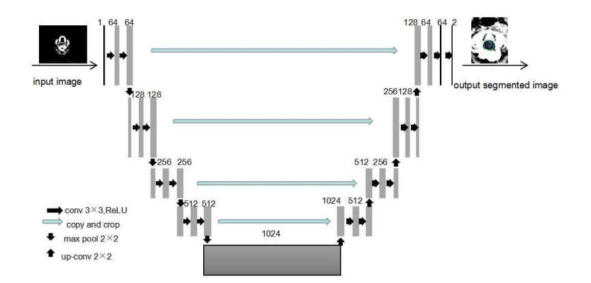
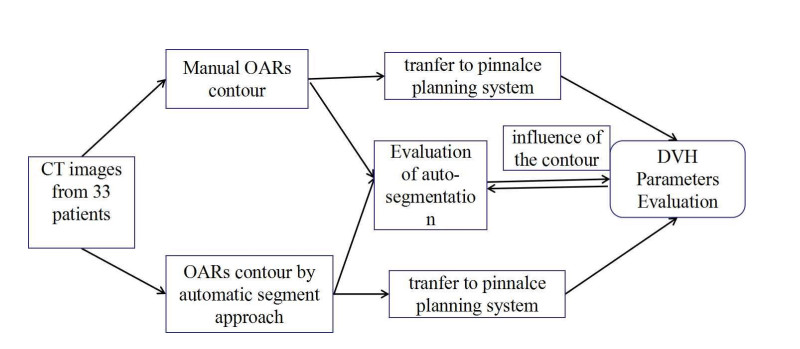
To evaluate the automatic segmentation approach for organ at risk (OARs) and compare the parameters of dose volume histogram (DVH) in radiotherapy. Methodology: Thirty-three patients were selected to contour OARs using automatic segmentation approach which based on U-Net, applying them to a number of the nasopharyngeal carcinoma (NPC), breast, and rectal cancer respectively. The automatic contours were transferred to the Pinnacle System to evaluate contour accuracy and compare the DVH parameters.

Results
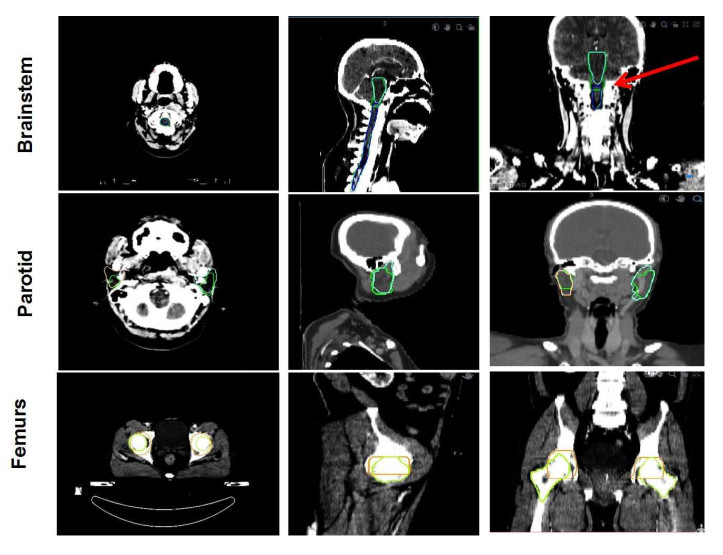
The time for manual contour was 56.5 ± 9, 23.12 ± 4.23 and 45.23 ± 2.39min for the OARs of NPC, breast and rectal cancer, and for automatic contour was 1.5 ± 0.23, 1.45 ± 0.78 and 1.8 ± 0.56 min. Automatic contours of Eye with the best Dice-similarity coefficients (DSC) of 0.907 ± 0.02 while with the poorest DSC of 0.459 ± 0.112 of Spinal Cord for NPC; And Lung with the best DSC of 0.944 ± 0.03 while with the poorest DSC of 0.709 ± 0.1 of Spinal Cord for breast; And Bladder with the best DSC of 0.91 ± 0.04 while with the poorest DSC of 0.43 ± 0.1 of Femoral heads for rectal cancer. The contours of Spinal Cord in H & N had poor results due to the division of the medulla oblongata. The contours of Femoral head, which different from what we expect, also due to manual contour result in poor DSC.

Conclusion
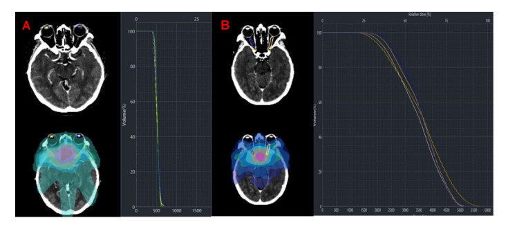
The automatic contour approach based deep learning method with sufficient accuracy for research purposes. However, the value of DSC does not fully reflect the accuracy of dose distribution, but can cause dose changes due to the changes in the OARs volume and DSC from the data. Considering the significantly time-saving and good performance in partial OARs, the automatic contouring also plays a supervisory role.
- automatic segment approach,
- deep Learning,
- organ at risk,
- intensity modulated radiotherapy,
- dose volume histogram
Citation: Han Zhou, Yikun Li, Ying Gu, Zetian Shen, Xixu Zhu, Yun Ge. A deep learning based automatic segmentation approach for anatomical structures in intensity modulation radiotherapy[J]. Mathematical Biosciences and Engineering, 2021, 18(6): 7506-7524. doi: 10.3934/mbe.2021371

Related Papers:

Abstract

Objective

To evaluate the automatic segmentation approach for organ at risk (OARs) and compare the parameters of dose volume histogram (DVH) in radiotherapy. Methodology: Thirty-three patients were selected to contour OARs using automatic segmentation approach which based on U-Net, applying them to a number of the nasopharyngeal carcinoma (NPC), breast, and rectal cancer respectively. The automatic contours were transferred to the Pinnacle System to evaluate contour accuracy and compare the DVH parameters.

Results

The time for manual contour was 56.5 ± 9, 23.12 ± 4.23 and 45.23 ± 2.39min for the OARs of NPC, breast and rectal cancer, and for automatic contour was 1.5 ± 0.23, 1.45 ± 0.78 and 1.8 ± 0.56 min. Automatic contours of Eye with the best Dice-similarity coefficients (DSC) of 0.907 ± 0.02 while with the poorest DSC of 0.459 ± 0.112 of Spinal Cord for NPC; And Lung with the best DSC of 0.944 ± 0.03 while with the poorest DSC of 0.709 ± 0.1 of Spinal Cord for breast; And Bladder with the best DSC of 0.91 ± 0.04 while with the poorest DSC of 0.43 ± 0.1 of Femoral heads for rectal cancer. The contours of Spinal Cord in H & N had poor results due to the division of the medulla oblongata. The contours of Femoral head, which different from what we expect, also due to manual contour result in poor DSC.

Conclusion

The automatic contour approach based deep learning method with sufficient accuracy for research purposes. However, the value of DSC does not fully reflect the accuracy of dose distribution, but can cause dose changes due to the changes in the OARs volume and DSC from the data. Considering the significantly time-saving and good performance in partial OARs, the automatic contouring also plays a supervisory role.

References

[1]	S. Li, J. Xiao, L. He, X. Yuan, The Tumor Target Segmentation of Nasopharyngeal Cancer in CT Images Based on Deep Learning Methods, Technol. Cancer Res. Treat., 18 (2019), 1533033819884561.
[2]	S. Gresswell, P. Renz, D. Werts, Y. Arshoun, Impact of Increasing Atlas Size on Accuracy of an Atlas-Based Auto-Segmentation Program (ABAS) for Organs-at-Risk (OARS) in Head and Neck (H & N) Cancer Patients, Int. J. Radiat. Oncol. Biol. Phys., 98 (2017), E31.
[3]	Y. Song, J. Hu, Q. Wu, F. Xu, S. Nie, Y. Zhao, et al., Automatic delineation of the clinical target volume and organs at risk by deep learning for rectal cancer postoperative radiotherapy, Radiother. Oncol., 145 (2020), 186-192. doi: 10.1016/j.radonc.2020.01.020
[4]	S. H. Ahn, A. U. Yeo, K. H. Kim, C. Kim, Y. Goh, S. Cho, et al., Comparative clinical evaluation of atlas and deep-learning-based auto-segmentation of organ structures in liver cancer, Radiat. Oncol., 14 (2019), 1-13. doi: 10.1186/s13014-018-1191-y
[5]	S. S. Mahdavi, S. E. Salcudean, W. J. Morris, I. Spandinger, A semi-automatic segmentation method for prostate boundary delineation, Brachytherapy, 8 (2009), P175.
[6]	L. Rundo, C. Militello, A. Tangherloni, G. Russo, S. Vitabile, M. C. Gilardi, et al., NeXt for neuro-radiosurgery: A fully automatic approach for necrosis extraction in brain tumor MRI using an unsupervised machine learning technique, Int. J. Imaging Syst. Technol., 28 (2018), 21-37. doi: 10.1002/ima.22253
[7]	X. Wang, H. Cui, G. Gong, Z. Fu, J. Zhou, J. Gu, et al., Computational delineation and quantitative heterogeneity analysis of lung tumor on 18F-FDG PET for radiation dose-escalation, Sci. Rep., 8 (2018), 10649. doi: 10.1038/s41598-018-28818-8
[8]	A. R. Eldesoky, E. S. Yates, T. B. Nyeng, M. S. Thomsen, H. M. Nielsen, et al., Internal and external validation of an ESTRO delineation guideline - dependent automated segmentation tool for loco-regional radiation therapy of early breast cancer, Radiother. Oncol., 121 (2016), 424-430. doi: 10.1016/j.radonc.2016.09.005
[9]	Z. Liu, X. Liu, H. Guan, H. Zhen, Y. Sun, Q. Chen, et al., Development and Validation of A Deep Learning Algorithm for Auto-Delineation of Clinical Target Volume and Organs at Risk in Cervical Cancer Radiotherapy, Radiother. Oncol., 153 (2020), 172-179. doi: 10.1016/j.radonc.2020.09.060
[10]	L. Li, D. Qi, Y. M. Jin, G. Q. Zhou, Y. Q. Tang, W. L. Chen, et al., Deep Learning for Automated Contouring of Primary Tumor Volumes by MRI for Nasopharyngeal Carcinoma, Radiol., 291 (2019), 677-686. doi: 10.1148/radiol.2019182012
[11]	O. Ronneberger, P. Fischer, T. Brox, U-Net: Convolutional Networks for Biomedical Image Segmentation, Int. Conf. Med. Image Comput. Comput.-Assist. Interv., (2015), 234-241.
[12]	A. V. Young, A. Wortham, I. Wernick, A. Evans, R. D. Ennis, Atlas-Based Segmentation Improves Consistency and Decreases Time Required for Contouring Postoperative Endometrial Cancer Nodal Volumes, Int. J. Radiat. Oncol. Biol. Phys., 79 (2011), 943-947. doi: 10.1016/j.ijrobp.2010.04.063
[13]	K. Brock, S. Mutic, T. Mcnutt, H. Li, M. L. Kessler, Use of image registration and fusion algorithms and techniques in radiotherapy: Report of the AAPM Radiation Therapy Committee Task Group No. 132, Med. Phys., 44 (2017), e43-e76.
[14]	S. H. Ahn, A. U. Yeo, K. H. Kim, C. Kim, Y. Goh, S. Cho, et al., Comparative clinical evaluation of atlas anddeep-learning-based auto-segmentation oforgan structures in liver cancer, Radiat. Oncol., 14 (2019), 1-13. doi: 10.1186/s13014-018-1191-y
[15]	N. T. C. Fung, W. M. Hung, C. K. Sze, M. C. H. Lee, W. T. Ng, Automatic segmentation for adaptive planning in nasopharyngeal carcinoma IMRT: Time, geometrical, and dosimetric analysis, Med. Dosim., 45 (2020), 60-65.
[16]	N. Lee, Q. Zhang, J. Kim, A. S. Garden, J. Mechalakos, K. Hu, et al., Phase II Study of Concurrent and Adjuvant Chemotherapy with Intensity Modulated Radiation Therapy (IMRT) or Three-dimensional Conformal Radiotherapy (3D-CRT) + Bevacizumab (BV) for Locally or Regionally Advanced Nasopharyngeal Cancer (NPC)[RTOG 0615]: Preliminary tocicity report, Int. J. Radiat. Oncol., Biol., Phys., 78 (2010), S103-S104.
[17]	J. Shi, Y. Ye, D. Zhu, L. Su, Y. Huang, J. Huang, Automatic Segmentation of Cardiac Magnetic Resonance Images based on Multi-input Fusion Network, Comput. Methods Programs Biomed., 209 (2021), 106323. doi: 10.1016/j.cmpb.2021.106323
[18]	Y. Ye, J. Shi, D. Zhu, L. Su, Y. Huang, J. Huang, Comparative analysis of pulmonary nodules segmentation using multiscale residual U-Net and fuzzy C-means clustering, Comput. Methods Programs Biomed., 209 (2021), 106332. doi: 10.1016/j.cmpb.2021.106332
[19]	G. E. Hinton, S. Osindero, Y. W. Teh, A Fast Learning Algorithm for Deep Belief Nets, Neural Comput., 18 (2014), 1527-1554.
[20]	S. Liang, F. Tang, X. Huang, K. Yang, T. Zhong, R. Hu, et al., Deep-learning-based detection and segmentation of organs at risk in nasopharyngeal carcinoma computed tomographic images for radiotherapy planning, Eur. Radiol., 29 (2019), 1961-1967. doi: 10.1007/s00330-018-5748-9
[21]	D. Shen, G. Wu, H. I. Suk, Deep Learning in Medical Image Analysis, Annu. Rev. Biomed. Eng., 19 (2017), 221-248. doi: 10.1146/annurev-bioeng-071516-044442
[22]	P. F. Christ, F. Ettlinger, F. Grun, M. E. A. Elshaera, J. Lipkova, S. Schlecht, et al., Automatic Liver and Lesion Segmentation in CT Using Cascaded Fully Convolutional Neural Networks and 3D Conditional Random Fields, Int. Confer. Med. Image Comput. Comput. Assist. Interv., (2016), 415-423.
[23]	D. Ciardo, M. A. Gerardi, S. Vigorito, A. Morra, V. Dell'Acqua, F. J. Diaz, et al., Atlas-based segmentation in breast cancer radiotherapy: Evaluation of specific and generic-purpose atlases, Breast, 32 (2017), 44-52. doi: 10.1016/j.breast.2016.12.010
[24]	A. Arsène-Henry, H. P. Xu, M. Robilliard, W. E. Amine, E. Costa, Y. M. Kirova, Evaluation of an automatic delineation software for organs at risk and lymph nodes in breast cancer, Radiother. Oncol., 22 (2018), 241-247.
[25]	M. La Macchia, F. Fellin, M. Amichetti, M. Cianchetti, S. Gianolini, V. Paola, et al., Systematic evaluation of three different commercial software solutions for automatic segmentation for adaptive therapy in head-and-neck, prostate and pleural cancer, Radiat. Oncol., 7 (2012), 160. doi: 10.1186/1748-717X-7-160
[26]	Z. Tang, G. Zhao, T. Ouyang, Two-phase deep learning model for short-term wind direction forecasting, Renew. Energ., 173 (2021), 1005-1016. doi: 10.1016/j.renene.2021.04.041
[27]	K. Wong, G. Fortino, D. Abbott, Deep learning-based cardiovascular image diagnosis: A promising challenge, Future Gener. Comput. Syst., 110 (2020), 802-811. doi: 10.1016/j.future.2019.09.047
[28]	L. Rundo, A. Stefano, C. Militello, G. Russo, M. G. Sabini, C. D''Arrigo, et al., A fully automatic approach for multimodal PET and MR image segmentation in Gamma Knife treatment planning, Comput. Methods Programs Biomed., 144 (2017), 77-96. doi: 10.1016/j.cmpb.2017.03.011
[29]	Q. Song, J. Bai, D. Han, S. Bhatia, W. Sun, W. Rockey, et al., Optimal co-segmentation of tumor in PET-CT images with context information, IEEE Trans. Med. Imaging, 32 (2013), 1685-1697. doi: 10.1109/TMI.2013.2263388
[30]	R. Kaderka, E. F. Gillespie, R. C. Mundt, A. K. Bryant, C. B. Sanudo, A. L. Harrison, et al., Geometric and dosimetric evaluation of atlas based auto-segmentation of cardiac structures in breast cancer patients, Radiother. Oncol., 131 (2019), 215-220. doi: 10.1016/j.radonc.2018.07.013
[31]	Y. Tong, Y. Yin, P. Cheng, G. Gong, Impact of deformable image registration on dose accumulation applied electrocardiograph-gated 4DCT in the heart and left ventricular myocardium during esophageal cancer radiotherapy, Radiat. Oncol., 13 (2018), 145. doi: 10.1186/s13014-018-1093-z
[32]	Q. Yang, H. Chao, D. Nguyen, S. Jiang, Mining Domain Knowledge: Improved Framework Towards Automatically Standardizing Anatomical Structure Nomenclature in Radiotherapy, IEEE Access, 8 (2020), 105286-105300. doi: 10.1109/ACCESS.2020.2999079
[33]	R. A. Mitchell, P. Wai, R. Colgan, A. M. Kirby, E. M. Donovan, Improving the efficiency of breast radiotherapy treatment planning using a semi-automated approach, J. Appl. Clin. Med. Phys., 18 (2017), 18-24.
[34]	H. P. Xu, A. Arsène-Henry, M. Robillard, M. Amessis, Y. Kirova, The use of new delineation tool "MIRADA" at the level of regional lymph nodes, step-by-step development and first results for early-stage breast cancer patients, Br. J. Radiol., 91 (2018), 20180095. doi: 10.1259/bjr.20180095

Reader Comments

Your name:*

Email:*
© 2021 the Author(s), licensee AIMS Press. This is an open access article distributed under the terms of the Creative Commons Attribution License (http://creativecommons.org/licenses/by/4.0)