Previous studies revealed that the epithelial component is associated with the modulation of the ovarian tumor microenvironment (TME). However, the identification of key transcriptional signatures of laser capture microdissected human ovarian cancer epithelia remains lacking.
We identified the differentially expressed transcriptional signatures of human ovarian cancer epithelia by meta-analysis of GSE14407, GSE2765, GSE38666, GSE40595, and GSE54388. Then we investigated the enrichment of KEGG pathways that are associated with epithelia-derived transcriptomes. Finally, we investigated the correlation of key epithelia-hub genes with the survival prognosis and immune infiltrations. Finally, we investigated the genetic alterations of key prognostic hub genes and their diagnostic efficacy in ovarian cancer epithelia.
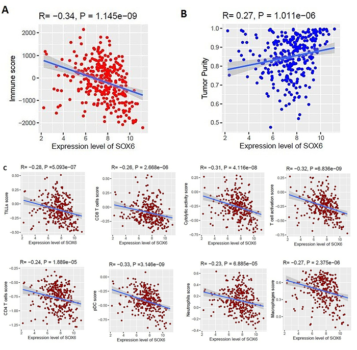
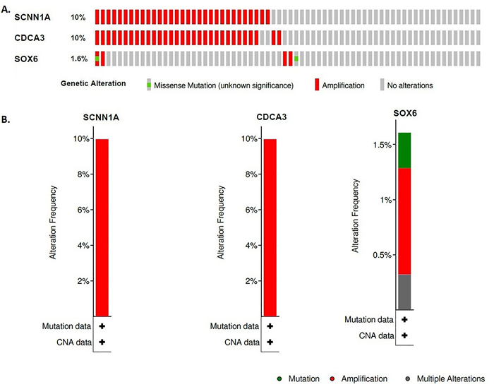
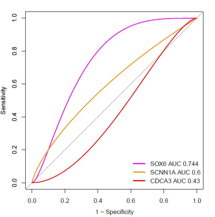
We identified 1339 differentially expressed genes (DEGs) in ovarian cancer epithelia including 541upregulated and 798 downregulated genes. We identified 21 (such as E2F4, FOXM1, TFDP1, E2F1, and SIN3A) and 11 (such as JUN, DDX4, FOSL1, NOC2L, and HMGA1) master transcriptional regulators (MTRs) that are interacted with upregulated and the downregulated genes in ovarian tumor epithelium, respectively. The STRING-based analysis identified hub genes (such as CDK1, CCNB1, AURKA, CDC20, and CCNA2) in ovarian cancer epithelia. The significant clusters of identified hub genes are associated with the enrichment of KEGG pathways including cell cycle, DNA replication, cytokine-cytokine receptor interaction, pathways in cancer, and focal adhesion. The upregulation of SCNN1A and CDCA3 and the downregulation of SOX6 are correlated with a shorter survival prognosis in ovarian cancer (OV). The expression level of SOX6 is negatively correlated with immune score and positively correlated with tumor purity in OV. Moreover, SOX6 is negatively correlated with the infiltration of TILs, CD8+ T cells, CD4+ Regulatory T cells, cytolytic activity, T cell activation, pDC, neutrophils, and macrophages in OV. Also, SOX6 is negatively correlated with various immune markers including CD8A, PRF1, GZMA, GZMB, NKG7, CCL3, and CCL4, indicating the immune regulatory efficiency of SOX6 in the TME of OV. Furthermore, SCNN1A, CDCA3, and SOX6 genes are genetically altered in OV and the expression levels of SCNN1A and SOX6 genes showed diagnostic efficacy in ovarian cancer epithelia.
The identified ovarian cancer epithelial-derived key transcriptional signatures are significantly correlated with survival prognosis and immune infiltrations, and may provide new insight into the diagnosis and treatment of epithelial ovarian cancer.
Citation: Dong-feng Li, Aisikeer Tulahong, Md. Nazim Uddin, Huan Zhao, Hua Zhang. Meta-analysis identifying epithelial-derived transcriptomes predicts poor clinical outcome and immune infiltrations in ovarian cancer[J]. Mathematical Biosciences and Engineering, 2021, 18(5): 6527-6551. doi: 10.3934/mbe.2021324
Previous studies revealed that the epithelial component is associated with the modulation of the ovarian tumor microenvironment (TME). However, the identification of key transcriptional signatures of laser capture microdissected human ovarian cancer epithelia remains lacking.
We identified the differentially expressed transcriptional signatures of human ovarian cancer epithelia by meta-analysis of GSE14407, GSE2765, GSE38666, GSE40595, and GSE54388. Then we investigated the enrichment of KEGG pathways that are associated with epithelia-derived transcriptomes. Finally, we investigated the correlation of key epithelia-hub genes with the survival prognosis and immune infiltrations. Finally, we investigated the genetic alterations of key prognostic hub genes and their diagnostic efficacy in ovarian cancer epithelia.
We identified 1339 differentially expressed genes (DEGs) in ovarian cancer epithelia including 541upregulated and 798 downregulated genes. We identified 21 (such as E2F4, FOXM1, TFDP1, E2F1, and SIN3A) and 11 (such as JUN, DDX4, FOSL1, NOC2L, and HMGA1) master transcriptional regulators (MTRs) that are interacted with upregulated and the downregulated genes in ovarian tumor epithelium, respectively. The STRING-based analysis identified hub genes (such as CDK1, CCNB1, AURKA, CDC20, and CCNA2) in ovarian cancer epithelia. The significant clusters of identified hub genes are associated with the enrichment of KEGG pathways including cell cycle, DNA replication, cytokine-cytokine receptor interaction, pathways in cancer, and focal adhesion. The upregulation of SCNN1A and CDCA3 and the downregulation of SOX6 are correlated with a shorter survival prognosis in ovarian cancer (OV). The expression level of SOX6 is negatively correlated with immune score and positively correlated with tumor purity in OV. Moreover, SOX6 is negatively correlated with the infiltration of TILs, CD8+ T cells, CD4+ Regulatory T cells, cytolytic activity, T cell activation, pDC, neutrophils, and macrophages in OV. Also, SOX6 is negatively correlated with various immune markers including CD8A, PRF1, GZMA, GZMB, NKG7, CCL3, and CCL4, indicating the immune regulatory efficiency of SOX6 in the TME of OV. Furthermore, SCNN1A, CDCA3, and SOX6 genes are genetically altered in OV and the expression levels of SCNN1A and SOX6 genes showed diagnostic efficacy in ovarian cancer epithelia.
The identified ovarian cancer epithelial-derived key transcriptional signatures are significantly correlated with survival prognosis and immune infiltrations, and may provide new insight into the diagnosis and treatment of epithelial ovarian cancer.

| [1] |
L. M. Hurwitz, P. F. Pinsky, B. Trabert, General population screening for ovarian cancer, Lancet, 397 (2021), 2128-2130. doi: 10.1016/S0140-6736(21)01061-8

|
| [2] |
R. L. Siegel, K. D. Miller, H. E. Fuchs, A. Jemal, Cancer statistics, 2021, CA Cancer J. Clin., 71 (2021), 7-33. doi: 10.3322/caac.21654
|
| [3] |
N. J. Bowen, L. D. Walker, L. V. Matyunina, S. Logani, K. A. Totten, B. B. Benigno, et al., Gene expression profiling supports the hypothesis that human ovarian surface epithelia are multipotent and capable of serving as ovarian cancer initiating cells, BMC Med. Genomics., 2 (2009), 71. doi: 10.1186/1755-8794-2-71
|
| [4] |
T. L. Yeung, C. S. Leung, K. K. Wong, G. Samimi, M. S. Thompson, J. Liu, et al., TGF-β modulates ovarian cancer invasion by upregulating CAF-derived versican in the tumor microenvironment, Cancer Res., 73 (2013), 5016-5028. doi: 10.1158/0008-5472.CAN-13-0023
|
| [5] |
J. Farley, L. L. Ozbun, M. J. Birrer, Genomic analysis of epithelial ovarian cancer, Cell Res., 18 (2008), 538-548. doi: 10.1038/cr.2008.52
|
| [6] | M. Ezzati, A. Abdullah, A. Shariftabrizi, J. Hou, M. Kopf, J. K. Stedman, et al., Recent advancements in prognostic factors of epithelial ovarian carcinoma, Int. Sch. Res. Not., 2014 (2014), e953509. |
| [7] |
M. L. Drakes, P. J. Stiff, Regulation of ovarian cancer prognosis by immune cells in the tumor microenvironment, Cancers, 10 (2018), 302. doi: 10.3390/cancers10090302
|
| [8] |
T. Gui, C. Yao, B. Jia, K. Shen, Identification and analysis of genes associated with epithelial ovarian cancer by integrated bioinformatics methods, PloS One, 16 (2021), e0253136. doi: 10.1371/journal.pone.0253136
|
| [9] |
J. Liu, H. Meng, S. Li, Y. Shen, H. Wang, W. Shan, et al., Identification of potential biomarkers in association with progression and prognosis in epithelial ovarian cancer by integrated bioinformatics analysis, Front. Genet., 10 (2019), 1031. doi: 10.3389/fgene.2019.01031
|
| [10] |
D. Matei, T. G. Graeber, R. L. Baldwin, B. Y. Karlan, J. Rao, D. D. Chang, Gene expression in epithelial ovarian carcinoma, Oncogene, 21 (2002), 6289-6298. doi: 10.1038/sj.onc.1205785
|
| [11] | P. Israelsson, E. Dehlin, I. Nagaev, E. Lundin, U. Ottander, L. Mincheva-Nilsson, Cytokine mRNA and protein expression by cell cultures of epithelial ovarian cancer-methodological considerations on the choice of analytical method for cytokine analyses, Am. J. Reprod. Immunol., 84 (2020), e13249. |
| [12] |
K. P. Prahm, C. K. Hø gdall, M. A. Karlsen, I. J. Christensen, G. W. Novotny, E. Hø gdall, MicroRNA characteristics in epithelial ovarian cancer, PloS One, 16 (2021), e0252401. doi: 10.1371/journal.pone.0252401
|
| [13] | A. A. Alshamrani, Roles of microRNAs in ovarian cancer tumorigenesis: two decades later, what have we learned?, Front. Oncol., 10 (2020), 1084. |
| [14] |
S. Udhaya Kumar, D. Thirumal Kumar, R. Bithia, S. Sankar, R. Magesh, M. Sidenna, et al., Analysis of differentially expressed genes and molecular pathways in familial hypercholesterolemia involved in atherosclerosis: a systematic and bioinformatics approach, Front. Genet., 11 (2020), 734. doi: 10.3389/fgene.2020.00734
|
| [15] |
J. Wan, S. Jiang, Y. Jiang, W. Ma, X. Wang, Z. He, et al., Corrigendum: data mining and expression analysis of differential lncRNA ADAMTS9-AS1 in prostate cancer, Front. Genet., 11 (2020), 361. doi: 10.3389/fgene.2020.00361
|
| [16] |
U. K. S., B. Rajan, T. K. D., A. P. V., T. Abunada, S. Younes, et al., Involvement of essential signaling cascades and analysis of gene networks in diabesity, Genes, 11 (2020), 1256. doi: 10.3390/genes11111256
|
| [17] |
D. Fu, B. Zhang, L. Yang, S. Huang, W. Xin, Development of an immune-related risk signature for predicting prognosis in lung squamous cell carcinoma, Front. Genet., 11 (2020), 978. doi: 10.3389/fgene.2020.00978
|
| [18] | E. R. King, C. S. Tung, Y. T. M. Tsang, Z. Zu, G. T. M. Lok, M. T. Deavers, et al, The anterior gradient homolog 3 (AGR3) gene is associated with differentiation and survival in ovarian cancer, Am. J. Surg. Pathol., 35 (2011), 904-912. |
| [19] |
C. Huang, E. A. Clayton, L. V. Matyunina, L. D. McDonald, B. B. Benigno, F. Vannberg, et al., Machine learning predicts individual cancer patient responses to therapeutic drugs with high accuracy, Sci. Rep., 8 (2018), 16444. doi: 10.1038/s41598-018-34753-5
|
| [20] | L. N. Lili, L. V. Matyunina, L. D. Walker, B. B. Benigno, J. F. McDonald, Molecular profiling predicts the existence of two functionally distinct classes of ovarian cancer stroma, BioMed Res. Int., 2013 (2013), 846387. |
| [21] |
T. L. Yeung, C. S. Leung, K. K. Wong, A. Gutierrez-Hartmann, J. Kwong, D. M. Gershenson, et al., ELF3 is a negative regulator of epithelial-mesenchymal transition in ovarian cancer cells, Oncotarget, 8 (2017), 16951-16963. doi: 10.18632/oncotarget.15208
|
| [22] | J. Xia, E. E. Gill, R. E. W. Hancock, NetworkAnalyst for statistical, visual and network-based meta-analysis of gene expression data, Nat. Protoc., 10 (2015), 823-844. |
| [23] | W. E. Johnson, C. Li, A. Rabinovic, Adjusting batch effects in microarray expression data using empirical Bayes methods, Biostat. Oxf. Engl., 8 (2007), 118-127. |
| [24] |
W. G. Cochran, The combination of estimates from different experiments, Biometrics, 10 (1954), 101-129. doi: 10.2307/3001666
|
| [25] | Y. Benjamini, Y. Hochberg, Controlling the false discovery rate: a practical and powerful approach to multiple testing, J. R. Stat. Soc. Ser. B Methodol., 57 (1995), 289-300. |
| [26] |
P. Shannon, A. Markiel, O. Ozier, N. S. Baliga, J. T. Wang, D. Ramage, et al., Cytoscape: a software environment for integrated models of biomolecular interaction networks, Genome Res., 13 (2003), 2498-2504. doi: 10.1101/gr.1239303
|
| [27] | R. Janky, A. Verfaillie, H. Imrichová, B. Van de Sande, L. Standaert, V. Christiaens, et al., iRegulon: from a gene list to a gene regulatory network using large motif and track collections, PLoS Comput. Biol., 10 (2014), e1003731. |
| [28] | J. Wang, Y. Wu, M. N. Uddin, R. Chen, J. P. Hao, Identification of potential key genes and regulatory markers in essential thrombocythemia through integrated bioinformatics analysis and clinical validation, Pharmacogenomics Pers. Med., 14 (2021), 767-784. |
| [29] |
A. Subramanian, P. Tamayo, V. K. Mootha, S. Mukherjee, B. L. Ebert, M. A. Gillette, et al., Gene set enrichment analysis: a knowledge-based approach for interpreting genome-wide expression profiles, Proc. Natl. Acad. Sci., 102 (2005), 15545-15550. doi: 10.1073/pnas.0506580102
|
| [30] | M. Kanehisa, M. Furumichi, M. Tanabe, Y. Sato, K. Morishima, KEGG: new perspectives on genomes, pathways, diseases and drugs, Nucleic Acids Res., 45 (2017), D353-D361. |
| [31] | D. Szklarczyk, A. L. Gable, D. Lyon, A. Junge, S. Wyder, J. Huerta-Cepas, et al., STRING v11: protein-protein association networks with increased coverage, supporting functional discovery in genome-wide experimental datasets, Nucleic Acids Res., 47 (2019), D607-D613. |
| [32] | C. H. Chin, S. H. Chen, H. H. Wu, C. W. Ho, M. T. Ko, C. Y. Lin, cytoHubba: identifying hub objects and sub-networks from complex interactome, BMC Syst. Biol., 8 (2014), S11. |
| [33] |
G. D. Bader, C. W. Hogue, An automated method for finding molecular complexes in large protein interaction networks, BMC Bioinformatics, 4 (2003), 2. doi: 10.1186/1471-2105-4-2
|
| [34] | T. Therneau, A package for survival analysis in R, 2021. Available from: https://cran.r-project.org/web/packages/survival/vignettes/survival.pdf. |
| [35] |
K. Yoshihara, M. Shahmoradgoli, E. Martínez, R. Vegesna, H. Kim, W. Torres-Garcia, et al., Inferring tumour purity and stromal and immune cell admixture from expression data, Nat. Commun., 4 (2013), 2612. doi: 10.1038/ncomms3612
|
| [36] |
S. Hä nzelmann, R. Castelo, J. Guinney, GSVA: gene set variation analysis for microarray and RNA-seq data, BMC Bioinformatics, 14 (2013), 7. doi: 10.1186/1471-2105-14-7
|
| [37] |
I. Tirosh, B. Izar, S. M. Prakadan, M. H. Wadsworth, D. Treacy, J. J. Trombetta, et al., Dissecting the multicellular ecosystem of metastatic melanoma by single-cell RNA-seq, Science, 352 (2016), 189-196. doi: 10.1126/science.aad0501
|
| [38] |
D. Aran, Z. Hu, A. J. Butte, xCell: digitally portraying the tissue cellular heterogeneity landscape, Genome Biol., 18 (2017), 220. doi: 10.1186/s13059-017-1349-1
|
| [39] | T. Davoli, H. Uno, E. C. Wooten, S. J. Elledge, Tumor aneuploidy correlates with markers of immune evasion and with reduced response to immunotherapy, Science, 355 (2017), eaaf8399. |
| [40] |
Z. Liu, M. Li, Z. Jiang, X. Wang, A comprehensive immunologic portrait of triple-negative breast cancer, Transl. Oncol., 11 (2018), 311-329. doi: 10.1016/j.tranon.2018.01.011
|
| [41] |
E. Cerami1, J. Gao, U. Dogrusoz, B. E. Gross, S. O. Sumer, B. A. Aksoy, et al., The cBio cancer genomics portal: an open platform for exploring multidimensional cancer genomics data, Cancer Discov., 2 (2012), 401-404. doi: 10.1158/2159-8290.CD-12-0095
|
| [42] |
X. Robin, N. Turck, A. Hainard, N. Tiberti, F. Lisacek, J. C. Sanchez, et al., pROC: an open-source package for R and S+ to analyze and compare ROC curves, BMC Bioinformatics, 12 (2011), 77. doi: 10.1186/1471-2105-12-77
|
| [43] | Q. Yang, R. Wang, B. Wei, C. Peng, L. Wang, G. Hu, et al., Candidate biomarkers and molecular mechanism investigation for glioblastoma multiforme utilizing WGCNA, BioMed Res. Int., 2018 (2018), e4246703. |
| [44] |
M. N. Uddin, R. Akter, M. Li, Z. Abdelrahman, Expression of SARS-COV-2 cell receptor gene ACE2 is associated with immunosuppression and metabolic reprogramming in lung adenocarcinoma based on bioinformatics analyses of gene expression profiles, Chem. Biol. Interact., 335 (2021), 109370. doi: 10.1016/j.cbi.2021.109370
|
| [45] | V. Gómez-Rubio, ggplot2 - elegant graphics for data analysis, J. Stat. Softw., 77 (2017), 1-3. |
| [46] | L. Zhao, Y. Li, Z. Zhang, J. Zou, J. Li, R. Wei, et al., Meta-analysis based gene expression profiling reveals functional genes in ovarian cancer, Biosci. Rep., 40 (2020), BSR20202911. |
| [47] | D. Chaves-Moreira, M. A. Mitchell, C. Arruza, P. Rawat, S. Sidoli, R. Nameki, et al., PAX8 orchestrates an angiogenic program through interaction with SOX17, preprint, BioRxiv, 2020.09.09.290387. |
| [48] |
X. Liu, Y. Gao, Y. Lu, J. Zhang, L. Li, F. Yin, Upregulation of NEK2 is associated with drug resistance in ovarian cancer, Oncol. Rep., 31 (2014), 745-754. doi: 10.3892/or.2013.2910
|
| [49] |
C. L. Au-Yeung, T. L. Yeung, A. Achreja, H. Zhao, K. P. Yip, S. Y. Kwan, et al., ITLN1 modulates invasive potential and metabolic reprogramming of ovarian cancer cells in omental microenvironment, Nat. Commun., 11 (2020), 3546. doi: 10.1038/s41467-020-17383-2
|
| [50] |
R. Januchowski, P. Zawierucha, M. Andrzejewska, M. Ruciński, M. Zabel, Microarray-based detection and expression analysis of ABC and SLC transporters in drug-resistant ovarian cancer cell lines, Biomed. Pharmacother., 67 (2013), 240-245. doi: 10.1016/j.biopha.2012.11.011
|
| [51] |
Y. Wang, F. Shao, L. Chen, ALDH1A2 suppresses epithelial ovarian cancer cell proliferation and migration by downregulating STAT3, OncoTargets Ther., 11 (2018), 599-608. doi: 10.2147/OTT.S145864
|
| [52] |
S. R. Rosario, M. D. Long, H. C. Affronti, A. M. Rowsam, K. H. Eng, D. J. Smiraglia, Pan-cancer analysis of transcriptional metabolic dysregulation using The Cancer Genome Atlas, Nat. Commun., 9 (2018), 5330. doi: 10.1038/s41467-018-07232-8
|
| [53] |
D. Reimer, S. Sadr, A. Wiedemair, S. Stadlmann, N. Concin, G. Hofstetter, et al. Clinical relevance of E2F family members in ovarian cancer-an evaluation in a training set of 77 patients, Clin. Cancer Res., 13 (2007), 144-151. doi: 10.1158/1078-0432.CCR-06-0780
|
| [54] |
L. Zhan, Y. Zhang, W. Wang, E. Song, Y. Fan, B. Wei, E2F1: a promising regulator in ovarian carcinoma, Tumor Biol., 37 (2016), 2823-2831. doi: 10.1007/s13277-015-4770-7
|
| [55] | S. Hein, S. Mahner, C. Kanowski, T. Lö ning, F. Jä nicke, K. Milde-Langosch, Expression of Jun and Fos proteins in ovarian tumors of different malignant potential and in ovarian cancer cell lines, Oncol. Rep., 22 (2009), 177-183. |
| [56] |
W. Yang, H. Cho, H. Y. Shin, J. Y. Chung, E. S. Kang, E. J. Lee, et al., Accumulation of cytoplasmic Cdk1 is associated with cancer growth and survival rate in epithelial ovarian cancer, Oncotarget, 7 (2016), 49481-49497. doi: 10.18632/oncotarget.10373
|
| [57] |
S. Wei, J. Liu, Y. Shi, X. Zhang, Y. Yang, Q. Song, Exploration of the sequential gene changes in epithelial ovarian cancer induced by carboplatin via microarray analysis, Mol. Med. Rep., 16 (2017), 3155-3160. doi: 10.3892/mmr.2017.7008
|
| [58] |
W. Li, Z. Liu, B. Liang, S. Chen, X. Zhang, X. Tong, et al., Identification of core genes in ovarian cancer by an integrative meta-analysis, J. Ovarian Res., 11 (2018), 94. doi: 10.1186/s13048-018-0467-z
|
| [59] | L. Wu, Z. H. Ling, H. Wang, X. Y. Wang, J. Gui, Upregulation of SCNN1A promotes cell proliferation, migration, and predicts poor prognosis in ovarian cancer through regulating epithelial-mesenchymal transformation, Cancer Biother. Radiopharm., 34 (2019), 642-649. |
| [60] |
C. Chen, S. Chen, M. Luo, H. Yan, L. Pang, C. Zhu, et al., The role of the CDCA gene family in ovarian cancer, Ann. Transl. Med., 8 (2020), 190. doi: 10.21037/atm.2020.01.99
|
| [61] | Y. Li, M. Xiao, F. Guo, The role of Sox6 and Netrin-1 in ovarian cancer cell growth, invasiveness, and angiogenesis, Tumour Biol., 39 (2017), 1010428317705508. |
| [62] | R. Aguirre-Gamboa, H. Gomez-Rueda, E. Martínez-Ledesma, A. Martínez-Torteya, R. Chacolla-Huaringa, A. Rodriguez-Barrientos, et al., SurvExpress: an online biomarker validation tool and database for cancer gene expression data using survival analysis, PloS One, 8 (2013), e74250. |
| [63] |
R. W. Tothill, A. V. Tinker, J. George, R. Brown, S. B. Fox, S. Lade, et al., Novel molecular subtypes of serous and endometrioid ovarian cancer linked to clinical outcome, Clin. Cancer Res., 14 (2008), 5198-5208. doi: 10.1158/1078-0432.CCR-08-0196
|
| [64] |
Y. Liu, Survival correlation of immune response in human cancers, Oncotarget, 10 (2019), 6885-6897. doi: 10.18632/oncotarget.27360
|
| [65] |
J. Wang, F. H. C. Cheng, J. Tedrow, W. Chang, C. Zhang, A. K. Mitra, Modulation of immune infiltration of ovarian cancer tumor microenvironment by specific subpopulations of fibroblasts, Cancers, 12 (2020), 3184. doi: 10.3390/cancers12113184
|
| [66] |
W. Wang, W. Zou, J. R. Liu, Tumor-infiltrating T cells in epithelial ovarian cancer: predictors of prognosis and biological basis of immunotherapy, Gynecol. Oncol., 151 (2018), 1-3. doi: 10.1016/j.ygyno.2018.09.005
|
| [67] | S. Lieber, S. Reinartz, H. Raifer, F. Finkernagel, T. Dreyer, H. Bronger, et al., Prognosis of ovarian cancer is associated with effector memory CD8+ T cell accumulation in ascites, CXCL9 levels and activation-triggered signal transduction in T cells, Oncoimmunology, 7 (2018), e1424672. |
| [68] |
S. U. Kumar, D. T. Kumar, R. Siva, C. G. P. Doss, H. Zayed, Integrative bioinformatics approaches to map potential novel genes and pathways involved in ovarian cancer, Front. Bioeng. Biotechnol., 7 (2019), 391. doi: 10.3389/fbioe.2019.00391
|
| [69] | S. Mishra, M. I. Shah, S. Udhaya Kumar, D. Thirumal Kumar, C. Gopalakrishnan, A. M. Al-Subaie, et al., Chapter Eleven - Network analysis of transcriptomics data for the prediction and prioritization of membrane-associated biomarkers for idiopathic pulmonary fibrosis (IPF) by bioinformatics approach, 123 (2020), 241-273. |
| [70] |
H. Yan, G. Zheng, J. Qu, Y. Liu, X. Huang, E. Zhang, et al., Identification of key candidate genes and pathways in multiple myeloma by integrated bioinformatics analysis, J. Cell. Physiol., 234 (2019), 23785-23797. doi: 10.1002/jcp.28947
|
| [71] |
S. Udhaya Kumar, D. Thirumal Kumar, R. Siva, C. George Priya Doss, S. Younes, N. Younes, et al., Dysregulation of signaling pathways due to differentially expressed genes from the B-cell transcriptomes of systemic lupus erythematosus patients-a bioinformatics approach, Front. Bioeng. Biotechnol., 8 (2020), 276. doi: 10.3389/fbioe.2020.00276
|
| [72] |
B. Charbonneau, E. L. Goode, K. R. Kalli, K. L. Knutson, M. S. DeRycke, The immune system in the pathogenesis of ovarian cancer, Crit. Rev. Immunol., 33 (2013), 137-164. doi: 10.1615/CritRevImmunol.2013006813
|
| [73] |
R. Nameki, H. Chang, J. Reddy, R. I. Corona, K. Lawrenson, Transcription factors in epithelial ovarian cancer: histotype-specific drivers and novel therapeutic targets, Pharmacol. Ther., 220 (2021), 107722. doi: 10.1016/j.pharmthera.2020.107722
|
| [74] | H. Ohtani, Focus on TILs: prognostic significance of tumor infiltrating lymphocytes in human colorectal cancer, Cancer Immun., 7 (2007), 4. |
| [75] |
D. Yang, Y. He, B. Wu, Y. Deng, N. Wang, M. Li, et al., Integrated bioinformatics analysis for the screening of hub genes and therapeutic drugs in ovarian cancer, J. Ovarian Res., 13 (2020), 10. doi: 10.1186/s13048-020-0613-2
|
| [76] |
H. Feng, Z. Y. Gu, Q. Li, Q. H. Liu, X. Y. Yang, J. J. Zhang, Identification of significant genes with poor prognosis in ovarian cancer via bioinformatical analysis, J. Ovarian Res., 12 (2019), 35. doi: 10.1186/s13048-019-0508-2
|
| [77] |
X. Yang, S. Zhu, L. Li, L. Zhang, S. Xian, Y. Wang, et al., Identification of differentially expressed genes and signaling pathways in ovarian cancer by integrated bioinformatics analysis, OncoTargets Ther., 11 (2018), 1457-1474. doi: 10.2147/OTT.S152238
|
 mbe-18-05-324-supplementary.xlsx mbe-18-05-324-supplementary.xlsx |
 |
Figures(7) / Tables(4)

Dong-feng Li, Aisikeer Tulahong, Md. Nazim Uddin, Huan Zhao, Hua Zhang. Meta-analysis identifying epithelial-derived transcriptomes predicts poor clinical outcome and immune infiltrations in ovarian cancer[J]. Mathematical Biosciences and Engineering, 2021, 18(5): 6527-6551. doi: 10.3934/mbe.2021324


 DownLoad: