SIR model-based verification of effect of COVID-19 Contact-Confirming Application (COCOA) on reducing infectors in Japan

Yuto Omae; Yohei Kakimoto; Jun Toyotani; Kazuyuki Hara; Yasuhiro Gon; Hirotaka Takahashi; Yuto Omae; Yohei Kakimoto; Jun Toyotani; Kazuyuki Hara; Yasuhiro Gon; Hirotaka Takahashi

doi:10.3934/mbe.2021323

Mathematical Biosciences and Engineering

2021, Volume 18, Issue 5: 6506-6526. doi: 10.3934/mbe.2021323

Previous Article Next Article

Research article Special Issues

SIR model-based verification of effect of COVID-19 Contact-Confirming Application (COCOA) on reducing infectors in Japan

1.
College of Industrial Technology, Nihon University, Izumi, Narashino, Chiba, Japan
2.
Nihon University School of Medicine, Ooyaguchi, Itabashi, Tokyo, Japan
3.
Research Center for Space Science, Advanced Research Laboratories, Tokyo City University, Todoroki, Setagaya, Tokyo, Japan

Received: 19 May 2021 Accepted: 29 June 2021 Published: 28 July 2021

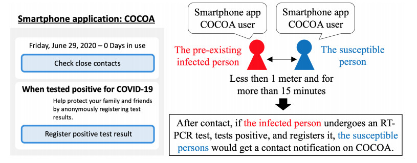
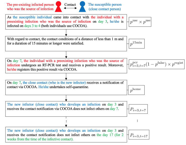
As of April 2021, the coronavirus disease (COVID-19) continues to spread in Japan. To overcome COVID-19, the Ministry of Health, Labor, and Welfare of the Japanese government developed and released the COVID-19 Contact-Confirming Application (COCOA) on June 19, 2020. COCOA users can know whether they have come into contact with infectors. If persons who receive a contact notification through COCOA undertake self-quarantine, the number of infectors in Japan will decrease. However, the effectiveness of COCOA in reducing the number of infectors depends on the usage rate of COCOA, the rate of fulfillment of contact condition, the rate of undergoing the reverse transcription polymerase chain reaction (RT-PCR) test, the false negative rate of the RT-PCR test, the rate of infection registration, and the self-quarantine rate. Therefore, we developed a Susceptible-Infected-Removed (SIR) model to estimate the effectiveness of COCOA. In this paper, we introduce the SIR model and report the simulation results for different scenarios that were assumed for Japan.
- contact tracing app,
- COCOA,
- COVID-19,
- SARS-CoV-2,
- SIR model,
- simulation in Japan
Citation: Yuto Omae, Yohei Kakimoto, Jun Toyotani, Kazuyuki Hara, Yasuhiro Gon, Hirotaka Takahashi. SIR model-based verification of effect of COVID-19 Contact-Confirming Application (COCOA) on reducing infectors in Japan[J]. Mathematical Biosciences and Engineering, 2021, 18(5): 6506-6526. doi: 10.3934/mbe.2021323

Related Papers:

Abstract

As of April 2021, the coronavirus disease (COVID-19) continues to spread in Japan. To overcome COVID-19, the Ministry of Health, Labor, and Welfare of the Japanese government developed and released the COVID-19 Contact-Confirming Application (COCOA) on June 19, 2020. COCOA users can know whether they have come into contact with infectors. If persons who receive a contact notification through COCOA undertake self-quarantine, the number of infectors in Japan will decrease. However, the effectiveness of COCOA in reducing the number of infectors depends on the usage rate of COCOA, the rate of fulfillment of contact condition, the rate of undergoing the reverse transcription polymerase chain reaction (RT-PCR) test, the false negative rate of the RT-PCR test, the rate of infection registration, and the self-quarantine rate. Therefore, we developed a Susceptible-Infected-Removed (SIR) model to estimate the effectiveness of COCOA. In this paper, we introduce the SIR model and report the simulation results for different scenarios that were assumed for Japan.

References

[1]	Ministry of Health, Labour, and Welfare, Request to install the COVID-19 contact-confirming application (COCOA) 2021, Available from: https://www.mhlw.go.jp/content/10900000/000773753.pdf.
[2]	Department of Health and Social Care, NHS. NHS COVID-19 App 2020, Available from: https://www.nhsx.nhs.uk/covid-19-response/nhs-covid-19-app/.
[3]	Anti-Covid-19 Tech Team, Trends in each country regarding the introduction of contact confirmation applications, 2020, Available from: https://cio.go.jp/sites/default/files/uploads/documents/techteam_20200508_02.pdf
[4]	F. Yang, Q. Yang, X. Liu, P. Wang, SIS evolutionary game model and multi-agent simulation of an infectious disease emergency, Technol. Health Care, 23 (2015), 603–613. doi: 10.3233/THC-150999
[5]	J. B. Dunham, An agent-based spatially explicit epidemiological model in MASON, J. Artif. Soc. Social Simul., 9 (2005).
[6]	H. Hirose, Pandemic simulations by MADE: A combination of multi-agent and differential equations, with a novel influenza a (H1N1) case, Information, 16 (2013), 5365–5390.
[7]	D. Chumachenko, V. Dobriak, M. Mazorchuk, I. Meniailov, K. Bazilevych, On agent-based approach to influenza and acute respiratory virus infection simulation, 14th International Conference on Advanced Trends in Radioelectronics, Telecommunications, and Computer Engineering, (2018), 192–195, doi: 10.1109/TCSET.2018.8336184
[8]	C. Hou, J. Chen, Y. Zhou, L. Hua, J. Yuan, S. He, et al., The effectiveness of quarantine in Wuhan city against coronavirus disease 2019 (COVID-19): a well-mixed SEIR model analysis, J. Med. Virol, 92 (2020), 841–848, doi: 10.1002/jmv.25827 doi: 10.1002/jmv.25827
[9]	B. Prasse, M. A. Achterberg, L. Ma, P. V. Mieghem, Network-inference-based prediction of the COVID-19 epidemic outbreak in the Chinese province Hubei, Appl. Network Sci., 5 (2020), doi: 10.1007/s41109-020-00274-2 doi: 10.1007/s41109-020-00274-2
[10]	Q. Yang, C. Yi, A. Vajdi, L. W. Cohnstaedt, H. Wu, X. Guo, et al., Short-term and long-term mitigation evaluations for the COVID-19 epidemic in Hubei province, China, Infect. Dis. Modell., 5 (2020), 563–574. doi: 10.1016/j.idm.2020.08.001
[11]	K. Chatterjee, K. Chatterjee, A. Kumar, S. Shankar, Healthcare impact of COVID-19 epidemic in India: a stochastic mathematical model, Med. J. Armed Forces India, 76 (2020), 147–155. doi: 10.1016/j.mjafi.2020.03.022
[12]	M. A. Achterberg, B. Prasse, L. Ma, S. Trajanovski, M. Kitsak, P. V. Mieghem, Comparing the accuracy of several network-based COVID-19 prediction algorithms, Int. J. Forecast., (2020), doi: 10.1016/j.ijforecast.2020.10.001
[13]	Z. Liu, P. Magal, G. Webb, Predicting the number of reported and unreported cases of COVID-19 epidemics in China, South Korea, Italy, France, Germany, and the United Kingdom, J. Theor. Biol, 509 (2020), doi: 10.1016/j.jtbi.2020.110501 doi: 10.1016/j.jtbi.2020.110501
[14]	E. A. Iboi, O. Sharomi, C. N. Ngonghala, A. B. Gumel, Mathematical modeling and analysis of COVID-19 pandemic in Nigeria, Math. Biosci. Eng., 17 (2020), 7192–7220, doi: 10.3934/mbe.2020369 doi: 10.3934/mbe.2020369
[15]	H. Wang, N. Yamamoto, Using a partial differential equation with Google Mobility data to predict COVID-19 in Arizona, Math. Biosci. Eng., 17 (2020), 4891–4904, doi: 10.3934/mbe.2020266 doi: 10.3934/mbe.2020266
[16]	S. Wang, Y. Liu, T. Hu, Examining the change of human mobility adherent to social restriction policies and its effect on COVID-19 cases in Australia, Int. J. Environ. Res. Public Health, 17 (2020), doi: 10.3390/ijerph17217930 doi: 10.3390/ijerph17217930
[17]	C. Zeng, J. Zhang, Z. Li, X. Sun, B. Olatosi, S. Weissman, X. Li, Spatial-temporal relationship between population mobility and COVID-19 outbreaks in South Carolina: time series forecasting analysis, J. Med. Internet Res., 23 (2021), doi:10.2196/27045 doi: 10.2196/27045
[18]	M. Sulyokab, M. D. Walker, Mobility and COVID-19 mortality across Scandinavia: A modeling study, Travel Med. Infect. Dis., 41 (2021), doi: 10.1016/j.tmaid.2021.102039 doi: 10.1016/j.tmaid.2021.102039
[19]	I. F. F. dos Santos, G. M. A. Almeida, F. A. B. F. de Moura, Adaptive SIR model for propagation of SARS-CoV-2 in Brazil, Phys. A, 569 (2021), doi: 10.1016/j.physa.2021.125773 doi: 10.1016/j.physa.2021.125773
[20]	I. F. F. dos Santos, G. M. A. Almeida, F. A. B. F. de Moura, Evolution of SARS-CoV-2 in the state of Alagoas-Brazil via an adaptive SIR model, Int. J. Mod. Phys. C, 32 (2021), doi: 10.1142/S0129183121500406 doi: 10.1142/S0129183121500406
[21]	M. Niwa, Y. Hara, S. Sengoku, K. Kodama, Effectiveness of social measures against COVID-19 outbreaks in several Japanese regions analyzed by system dynamic modeling, SSRN 3653579 (2020), doi: 10.2139/ssrn.3653579
[22]	S. Kurahashi, Estimating effectiveness of preventing measures for 2019 novel coronavirus diseases (COVID-19), Trans. Jpn. Soc. Artif. Intell., 35 (2020), D-K28-1, doi: 10.1527/tjsai.D-K28 doi: 10.1527/tjsai.D-K28
[23]	G. L. Vasconcelos, A. M. S. Macêdo, G. C. Duarte-Filho, A. A. Brum, R. Ospina, F. A. G. Almeida, Power law behaviour in the saturation regime of fatality curves of the COVID-19 pandemic, Sci. Rep., 11 (2021), article number: 4619, doi: 10.1038/s41598-021-84165-1 doi: 10.1038/s41598-021-84165-1
[24]	A. M. S. Macêdo, A. A. Brum, G. C. Duarte-Filho, F. A. G. Almeida, R. Ospina, G. L. Vasconcelos, A comparative analysis between a SIRD compartmental model and the Richards growth model, medRxiv, doi: 10.1101/2020.08.04.20168120
[25]	R. Hinch, W. Probert, A. Nurtay, M. Kendall, C. Wymant, M. Hall, et al., Effective configurations of a digital contact tracing app: a report to NHSX, 2020. Available from: https://045.medsci.ox.ac.uk/files/files/report-effective-app-configurations.pdf.
[26]	E. Hernandez-Orallo, P. Manzoni, C. T. Calafate, J. C. Cano, Evaluating how smartphone contact tracing technology can reduce the spread of infectious diseases: The case of COVID-19, IEEE Access, 8 (2020), 99083–99097. doi: 10.1109/ACCESS.2020.2998432
[27]	M. E. Kretzschmar, G. Rozhnova, M. C. J. Bootsma, M. Boven, J. H. H. M. Wijgert, M. J. M. Bonten, Impact of delays on effectiveness of contact tracing strategies for COVID-19: A modeling study, Lancet Public Health, 5 (2020), e452–e459. doi: 10.1016/S2468-2667(20)30157-2
[28]	J. A. Kucharski, P. Klepac, A. J. K. Conlan, S. M. Kissler, M. L. Tang, H. Fry, et al., Effectiveness of isolation, testing, contact tracing, and physical distancing on reducing transmission of SARS-CoV-2 in different settings: A mathematical modeling study, Lancet Infect. Dis., 20 (2020), 1151–1160. doi: 10.1016/S1473-3099(20)30457-6
[29]	L. Ferretti, C. Wymant, M. Kendall, L. Zhao, A. Nurtay, L. Abeler-Dorner, et al., Quantifying SARS-CoV-2 transmission suggests epidemic control with digital contact tracing, Science, 368 (2020), doi: 10.1126/science.abb6936 doi: 10.1126/science.abb6936
[30]	Y. Omae, J. Toyotani, K. Hara, H. Takahashi, Effectiveness of COVID-19 contact-confirming application (COCOA) based on a multi-agent simulation, preprint, arXiv: 2008.13166.
[31]	J. Kurita, T. Sugawara, Y. Ohkusa, Effectiveness of COCOA, a COVID-19 contact notification application, in Japan, preprint, medRxiv (2020) doi: 10.1101/2020.07.11.20151597
[32]	G. Kobayashi, S. Sugasawa, H. Tamae, T. Ozu, Predicting intervention effect for COVID-19 in Japan: State space modeling approach, Biosci. Trends, 14 (2020), 174–181, doi: 10.5582/bst.2020.03133 doi: 10.5582/bst.2020.03133
[33]	M. S. Boudrioua, A. Boudrioua, Predicting the COVID-19 epidemic in algeria using the SIR model, preprint, medrxiv (2020) doi: 10.1101/2020.04.25.20079467
[34]	B. Malavika, S. Marimuthu, M. Joy, A. Nadaraj, E. S. Asirvatham, L. Jeyaseelan, Forecasting COVID-19 epidemic in India and high incidence states using SIR and logistic growth models, Clin. Epidemiol. Glob. Health, 9 (2020), 26–33.
[35]	I. Cooper, A. Mondal, C. G. Antonopoulos, A SIR Model Assumption for the spread of COVID-19 in different communities, Chaos Solitons Fractals, 139 (2020), doi: 10.1016/j.chaos.2020.110057 doi: 10.1016/j.chaos.2020.110057
[36]	G. Nakamura, B. Grammaticos, M. Badoual, Confinement strategies in a simple SIR Model, Regul. Chaot. Dyn., 25 (2020), 509–521. doi: 10.1134/S1560354720060015
[37]	M. Itakura, M. Asahi, T. Yamaguchi, Proposal of an infection model for foot-and-mouth disease epidemic, Oper. Res. Manag. Sci. Res., 56 (2011), 728–734, Available from: http://www.orsj.or.jp/archive2/or56-12/or56-12_728.pdf
[38]	H. Nishiura, H. Inaba, Prediction of infectious disease outbreak with particular emphasis on statistical issues using the transmission model, Proc. Inst. Stat. Math., 54 (2006), 461–480, Available from: https://www.ism.ac.jp/editsec/toukei/pdf/54-2-461.pdf
[39]	T. Tsuchiya, A study on the spread of new coronavirus infections, Commun. Oper. Res. Soc. Jpn., 66 (2021), 90–103, doi: 10.24545/00001758 doi: 10.24545/00001758
[40]	Ministry of Health, Labour, and Welfare, Open data of positive result of COVID-19, 2021, Available from: https://www.mhlw.go.jp/content/pcr_positive_daily.csv.
[41]	Ministry of Health, Labour, and Welfare, COVID-19 Contact-Confirming Application (COCOA), 2020, Available from: https://www.mhlw.go.jp/stf/seisakunitsuite/bunya/cocoa_00138.html.
[42]	L. M. Kucirka, S. A. Lauer, O. Laeyendecker, D. Boon, J. Lessler, Variation in false-negative rate of reverse transcriptase polymerase Chain reaction-based SARS-CoV-2 tests by time since exposure, Ann. Intern. Med., 173 (2020), 262–267. doi: 10.7326/M20-1495
[43]	Python 3.7.3, 2019, Available from: https://www.python.org/downloads/release/python-373/
[44]	Numpy, 2021, Available from: https://numpy.org
[45]	E. B. Postnikov, Estimation of COVID-19 dynamics "on a back-of-envelope": Does the simplest SIR model provide quantitative parameters and predictions?, Chaos Solitons Fractals, 135 (2020), doi: 10.1016/j.chaos.2020.109841

Reader Comments

Your name:*

Email:*
© 2021 the Author(s), licensee AIMS Press. This is an open access article distributed under the terms of the Creative Commons Attribution License (http://creativecommons.org/licenses/by/4.0)