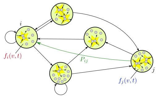
In this paper, we propose a Boltzmann-type kinetic model of the spreading of an infectious disease on a network. The latter describes the connections among countries, cities or districts depending on the spatial scale of interest. The disease transmission is represented in terms of the viral load of the individuals and is mediated by social contacts among them, taking into account their displacements across the nodes of the network. We formally derive the hydrodynamic equations for the density and the mean viral load of the individuals on the network and we analyse the large-time trends of these quantities with special emphasis on the cases of blow-up or eradication of the infection. By means of numerical tests, we also investigate the impact of confinement measures, such as quarantine or localised lockdown, on the diffusion of the disease on the network.
Citation: Nadia Loy, Andrea Tosin. A viral load-based model for epidemic spread on spatial networks[J]. Mathematical Biosciences and Engineering, 2021, 18(5): 5635-5663. doi: 10.3934/mbe.2021285
In this paper, we propose a Boltzmann-type kinetic model of the spreading of an infectious disease on a network. The latter describes the connections among countries, cities or districts depending on the spatial scale of interest. The disease transmission is represented in terms of the viral load of the individuals and is mediated by social contacts among them, taking into account their displacements across the nodes of the network. We formally derive the hydrodynamic equations for the density and the mean viral load of the individuals on the network and we analyse the large-time trends of these quantities with special emphasis on the cases of blow-up or eradication of the infection. By means of numerical tests, we also investigate the impact of confinement measures, such as quarantine or localised lockdown, on the diffusion of the disease on the network.

| [1] |
A. Wesolowski, E. zu Erbach-Schoenberg, A. J. Tatem, C. Lourenço, C. Viboud, V. Charu, et al., Multinational patterns of seasonal asymmetry in human movement influence infectious disease dynamics, Nat. Commun., 8 (2017), 1–9. doi: 10.1038/s41467-016-0009-6

|
| [2] | W. O. Kermack, A. G. McKendrick, Contributions to the mathematical theory of epidemics–I, Bull. Math. Biol., 53 (1991), 33–55. |
| [3] |
V. Colizza, A. Vespignani, Epidemic modeling in metapopulation systems with heterogeneous coupling pattern: Theory and simulations, J. Theor. Biol., 251 (2008), 450–467. doi: 10.1016/j.jtbi.2007.11.028
|
| [4] | M. J. Keeling, K. T. D. Eames, Networks and epidemic models, J. R. Soc. Interface, 2 (2005), 295–307. |
| [5] | G. Bertaglia, L. Pareschi, Hyperbolic models for the spread of epidemics on networks: kinetic description and numerical methods, ESAIM Math. Model. Numer. Anal., 55 (2020), 381–407. |
| [6] | W. Boscheri, G. Dimarco, L. Pareschi, Modeling and simulating the spatial spread of an epidemic through multiscale kinetic transport equations, preprint, arXiv: 2012.10101. |
| [7] | L. Almeida, P. A. Bliman, G. Nadin, B. Perthame, N. Vauchelet, Final size and convergence rate for an epidemic in heterogeneous population, preprint, arXiv: 2010.1541. |
| [8] | M. Martcheva, An Introduction to Mathematical Epidemiology, Springer, 2015. |
| [9] | A. Apolloni, C. Poletto, J. J. Ramasco, P. Jensen, V. Colizza, Metapopulation epidemic models with heterogeneous mixing and travel behaviour, Theor. Biol. Med. Model., 11 (2014), 1–26. |
| [10] | F. Arrigoni, A. Pugliese, Global stability of equilibria for a metapopulation S-I-S model, in Math Everywhere (eds. G. Aletti, A. Micheletti, D. Morale and M. Burger), Springer, 2007,229–240. |
| [11] |
A. D. Barbour, A. Pugliese, Convergence of a structured metapopulation model to Levins's model, J. Math. Biol., 49 (2004), 468–500. doi: 10.1007/s00285-004-0272-8
|
| [12] |
R. Pastor-Satorras, C. Castellano, P. Van Mieghem, A. Vespignani, Epidemic processes in complex networks, Rev. Modern Phys., 87 (2015), 925–979. doi: 10.1103/RevModPhys.87.925
|
| [13] | L. Zino, M. Cao, Analysis, prediction, and control of epidemics: A survey from scalar to dynamic network models, preprint: arXiv: 2013.00181. |
| [14] | F. Parino, L. Zino, M. Porfiri, A. Rizzo, Modelling and predicting the effect of social distancing and travel restrictions on COVID-19 spreading, preprint: arXiv: 2010.05968. |
| [15] | M. Garavello, K. Han, B. Piccoli, Models for Vehicular Traffic on Networks, Am. Inst. Math. Sci., 2016 (2016). |
| [16] | M. Garavello, B. Piccoli, Traffic Flow on Networks–Conservation Laws Models, Am. Inst. Math. Sci., 2016 (2016). |
| [17] |
G. Dimarco, L. Pareschi, G. Toscani, M. Zanella, Wealth distribution under the spread of infectious diseases, Phys. Rev. E, 102 (2020), 022303. doi: 10.1103/PhysRevE.102.022303
|
| [18] | G. Dimarco, B. Perthame, G. Toscani, M. Zanella, Kinetic models for epidemic dynamics with social heterogeneity, preprint: arXiv: 2009.01140. |
| [19] |
D. B. Larremore, B. Wilder, E. Lester, S. Shehata, J. M. Burke, J. A. Hay, et al., Test sensitivity is secondary to frequency and turnaround time for COVID-19 screening, Sci. Adv., 7 (2021), eabd5393. doi: 10.1126/sciadv.abd5393
|
| [20] |
M. L. Bertotti, G. Modanese, Discretized kinetic theory on scale-free networks, Eur. Phys. J. Special Topics, 225 (2016), 1879–1891. doi: 10.1140/epjst/e2015-50119-6
|
| [21] | M. Burger, Network structured kinetic models of social interactions, Vietnam J. Math., 2021 (2021), 1–20. |
| [22] |
N. Lanchier, Rigorous proof of the Boltzmann-Gibbs distribution of money on connected graphs, J. Stat. Phys., 167 (2017), 160–172. doi: 10.1007/s10955-017-1744-8
|
| [23] |
N. Lanchier, S. Reed, Rigorous results for the distribution of money on connected graphs, J. Stat. Phys., 171 (2018), 727–743. doi: 10.1007/s10955-018-2024-y
|
| [24] | N. Loy, A. Tosin, Boltzmann-type equations for multi-agent systems with label switching, Forthcoming, 2021. |
| [25] | L. Pareschi, G. Toscani, Interacting Multiagent Systems: Kinetic equations and Monte Carlo methods, Oxford University Press, 2013. |
| [26] | H. Minc, Nonnegative matrices, Wiley-Interscience, 1988. |
| [27] |
B. Espinoza, C. Castillo-Chavez, C. Perrings, Mobility restrictions for the control of epidemics: When do they work?, PLoS ONE, 15 (2020), e0235731. doi: 10.1371/journal.pone.0235731
|
Figures(7) / Tables(1)

Nadia Loy, Andrea Tosin. A viral load-based model for epidemic spread on spatial networks[J]. Mathematical Biosciences and Engineering, 2021, 18(5): 5635-5663. doi: 10.3934/mbe.2021285


 DownLoad: