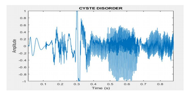
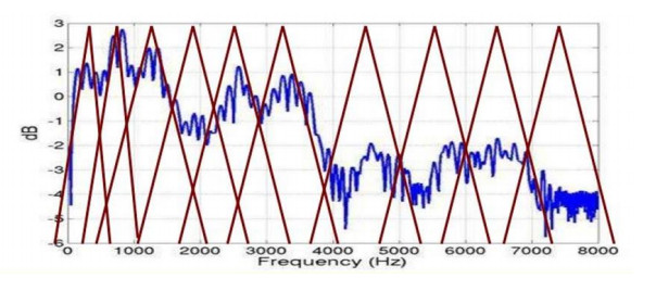
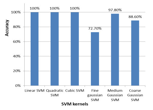
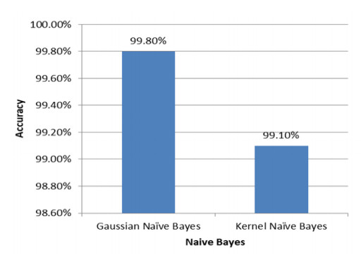
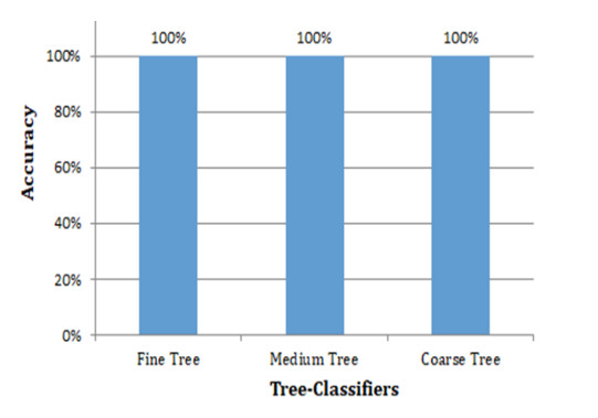
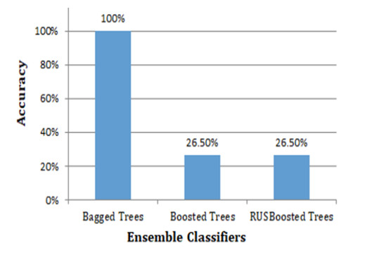
Voice pathologies are irregular vibrations produced due to vocal folds and various factors malfunctioning. In medical science, novel machine learning algorithms are applied to construct a system to identify disorders that occur invoice. This study aims to extract the features from the audio signals of four chosen diseases from the SVD dataset, such as laryngitis, cyst, non-fluency syndrome, and dysphonia, and then compare the four results of machine learning algorithms, i.e., SVM, Naïve Byes, decision tree and ensemble classifier. In this project, we have used a comparative approach along with the new combination of features to detect voice pathologies which are laryngitis, cyst, non-fluency syndrome, and dysphonia from the SVD dataset. The combination of specific 13 MFCC (mel-frequency cepstral coefficients) features along with pitch, zero crossing rate (ZCR), spectral flux, spectral entropy, spectral centroid, spectral roll-off, and short term energy for more accurate detection of voice pathologies. It is proven that the combination of features extracted gives the best product on the audio, which split into 10 ms. Four machine learning classifiers, SVM, Naïve Bayes, decision tree and ensemble classifier for the inter classifier comparison, give 93.18, 99.45,100 and 51%, respectively. Out of these accuracies, both Naïve Bayes and the decision tree show the most promising results with a higher detection rate. Naïve Bayes and decision tree gives the highest reported outcomes on the selected set of features in the proposed methodology. The SVM has also been concluded to be the commonly used voice condition identification algorithm.
Citation: Sidra Abid Syed, Munaf Rashid, Samreen Hussain, Anoshia Imtiaz, Hamnah Abid, Hira Zahid. Inter classifier comparison to detect voice pathologies[J]. Mathematical Biosciences and Engineering, 2021, 18(3): 2258-2273. doi: 10.3934/mbe.2021114
Voice pathologies are irregular vibrations produced due to vocal folds and various factors malfunctioning. In medical science, novel machine learning algorithms are applied to construct a system to identify disorders that occur invoice. This study aims to extract the features from the audio signals of four chosen diseases from the SVD dataset, such as laryngitis, cyst, non-fluency syndrome, and dysphonia, and then compare the four results of machine learning algorithms, i.e., SVM, Naïve Byes, decision tree and ensemble classifier. In this project, we have used a comparative approach along with the new combination of features to detect voice pathologies which are laryngitis, cyst, non-fluency syndrome, and dysphonia from the SVD dataset. The combination of specific 13 MFCC (mel-frequency cepstral coefficients) features along with pitch, zero crossing rate (ZCR), spectral flux, spectral entropy, spectral centroid, spectral roll-off, and short term energy for more accurate detection of voice pathologies. It is proven that the combination of features extracted gives the best product on the audio, which split into 10 ms. Four machine learning classifiers, SVM, Naïve Bayes, decision tree and ensemble classifier for the inter classifier comparison, give 93.18, 99.45,100 and 51%, respectively. Out of these accuracies, both Naïve Bayes and the decision tree show the most promising results with a higher detection rate. Naïve Bayes and decision tree gives the highest reported outcomes on the selected set of features in the proposed methodology. The SVM has also been concluded to be the commonly used voice condition identification algorithm.

| [1] | P. Harar, J. B. Alonso-Hernandezy, J. Mekyska, Z. Galaz, R. Burget, Z. Smekal, Voice pathology detection using deep learning: a preliminary study, in 2017 international conference and workshop on bioinspired intelligence (IWOBI), (2017), 1-4. |
| [2] |
M. Alhussein, G. Muhammad, Voice pathology detection using deep learning on mobile healthcare framework, IEEE Access, 6 (2018), 41034-41041. doi: 10.1109/ACCESS.2018.2856238

|
| [3] |
F. Teixeira, J. Fernandes, V. Guedes, A. Junior, J. P. Teixeira, Classification of control/pathologic subjects with support vector machines, Procedia Comput. Sci., 138 (2018), 272-279. doi: 10.1016/j.procs.2018.10.039
|
| [4] |
V. Guedes, A. Junior, J. Fernandes, F. Teixeira, J. P. Teixeira, Long short term memory on chronic laryngitis classification, Procedia Comput. Sci., 138 (2018), 250-257. doi: 10.1016/j.procs.2018.10.036
|
| [5] |
J. P. Teixeira, P. O. Fernandes, N. Alves, Vocal acoustic analysis-classification of dysphonic voices with artificial neural networks, Procedia Comput. Sci., 121 (2017), 19-26. doi: 10.1016/j.procs.2017.11.004
|
| [6] |
J. Kreiman, B. R. Gerratt, K. Precoda, Listener experience and perception of voice quality, J. Speech, Lang., Hear. Res., 33 (1990), 103-115. doi: 10.1044/jshr.3301.103
|
| [7] |
G. Muhammad, G. Altuwaijri, M. Alsulaiman, Z. Ali, T. A. Mesallam, M. Farahat, et al., Automatic voice pathology detection and classification using vocal tract area irregularity, Biocybern. Biomed. Eng., 36 (2016), 309-317. doi: 10.1016/j.bbe.2016.01.004
|
| [8] | N. Rezaei, A. Salehi, An introduction to speech sciences (acoustic analysis of speech), Iran. Rehabil. J., 4 (2006), 5-14. |
| [9] | J. W. Lee, H. G. Kang, J. Y. Choi, Y. I. Son, An investigation of vocal tract characteristics for acoustic discrimination of pathological voices, BioMed Res. Int., 2013 (2013). |
| [10] | US Department of Health and Human Services, NIDCD fact sheet: Speech and language developmental milestones, NIH Publication, 2010. |
| [11] |
S. A. Syed, M. Rashid, S. Hussain, Meta-analysis of voice disorders databases and applied machine learning techniques, Math. Biosci. Eng., 17 (2020), 7958-7979. doi: 10.3934/mbe.2020404
|
| [12] | B. Boyanov, S. Hadjitodorov, Acoustic analysis of pathological voices. A voice analysis system for the screening of laryngeal diseases, IEEE Eng. Med. Biol. Mag., 16 (1997), 74-82. |
| [13] | A. Zulfiqar, A. Muhammad, A. M. Enriquez, A speaker identification system using MFCC features with VQ technique, in 2009 Third International Symposium on Intelligent Information Technology Application, IEEE, 3 (2009), 115-118. |
| [14] | A. Al-Nasheri, G. Muhammad, M. Alsulaiman, Z. Ali, K. H. Malki, T. A. Mesallam, et al., Voice pathology detection and classification using auto-correlation and entropy features in different frequency regions, IEEE Access, 6 (2017), 6961-6974. |
| [15] | A. Al-Nasheri, G. Muhammad, M. Alsulaiman, Z. Ali, T. A. Mesallam, M. Farahat, et al., An investigation of multidimensional voice program parameters in three different databases for voice pathology detection and classification, J. Voice, 31 (2017), 113.e9-e18. |
| [16] |
A. Al-Nasheri, G. Muhammad, M. Alsulaiman, Z. Ali, Investigation of voice pathology detection and classification on different frequency regions using correlation functions, J. Voice, 31 (2017), 3-15. doi: 10.1016/j.jvoice.2016.01.014
|
| [17] |
F. Teixeira, J. Fernandes, V. Guedes, A. Junior, J. P. Teixeira, Classification of control/pathologic subjects with support vector machines, Proced. Comput. Sci., 138 (2018), 272-279. doi: 10.1016/j.procs.2018.10.039
|
| [18] |
J. P. Teixeira, P. O. Fernandes, N. Alves, Vocal acoustic analysis-classification of dysphonic voices with artificial neural networks, Proced. Comput. Sci., 121 (2017), 19-26. doi: 10.1016/j.procs.2017.11.004
|
| [19] | E. S. Fonseca, R. C. Guido, S. B. Junior, H. Dezani, R. R. Gati, D. C. Pereira, Acoustic investigation of speech pathologies based on the discriminative paraconsistent machine (DPM), Biomed. Signal Process. Control, 55 (2020). |
| [20] | Z. Ali, M. Alsulaiman, G. Muhammad, I. Elamvazuthi, A. Al-nasheri, T. A. Mesallam, et al., Intra-and inter-database study for Arabic, English, and German databases: do conventional speech features detect voice pathology?, J. Voice, 31 (2017), 386.e1-e8. |
| [21] | S. Kadiri, P. Alku, Analysis and detection of pathological voice using glottal source features, IEEE J. Sel. Top. Signal Process., 14 (2019), 367-379. |
| [22] | B. Woldert-Jokisz, Saarbruecken Voice Database, 2007. Available from: http://www.stimmdatenbank.coli.uni-saarland.de/help_en.php4. |
| [23] | S. Huang, N. Cai, P. P. Pacheco, S. Narrandes, Y. Wang, W. Xu, Applications of support vector machine (SVM) learning in cancer genomics, Cancer Genomics-Proteomics, 15 (2018), 41-51. |
| [24] | A. Shmilovici, Support vector machines, in Data Mining and Knowledge Discovery Handbook, Springer, Boston, MA, (2009), 231-247. |
| [25] |
W. Zhang, F. Gao, An improvement to naive bayes for text classification, Procedia Eng., 15 (2011), 2160-2164. doi: 10.1016/j.proeng.2011.08.404
|
| [26] | C. C. Aggarwal, Data Mining: The Textbook, Springer, 2015. |
| [27] | L. Toth, A. Kocsor, J. Csirik, On naive Bayes in speech recognition, Int. J. Appl. Math. Comput. Sci., 15 (2005), 287-294. |
| [28] |
C. Kingsford, S. Salzberg, What are decision trees?, Nat. Biotechnol., 26 (2008), 1011-1013. doi: 10.1038/nbt0908-1011
|
| [29] | T. G. Dietterich, Ensemble methods in machine learning, in International workshop on multiple classifier systems, Springer, Berlin, Heidelberg, (2000), 1-15. |
| [30] |
E. Bauer, R. Kohavi, An empirical comparison of voting classification algorithms: Bagging, boosting, and variants, Mach. Learn., 36 (1999), 105-139. doi: 10.1023/A:1007515423169
|
| [31] | R. Sharma, K. Hara, H. Hirayama, A machine learning and cross-validation approach for the discrimination of vegetation physiognomic types using satellite based multispectral and multitemporal data, Scientifica, 2017 (2017), 9806479. |
| [32] | R. O. Duda, P. E. Hart, D. G. Stork, Pattern Classification, 2nd edition, Wiley-Interscience, USA, 2000. |
| [33] | S. Memon, M. Lech, L. He, Using information theoretic vector quantization for inverted MFCC based speaker verification, in 2009 2nd International Conference on Computer, Control and Communication, IEEE, (2009), 1-5. |
| [34] | M. Sahidullah, G. Saha, On the use of distributed dct in speaker identification, in 2009 Annual IEEE India Conference, IEEE, (2009), 1-4. |
| [35] | Ö. Eskidere, A. Gürhanlı, Voice disorder classification based on multitaper mel frequency cepstral coefficients features, Comput. Math. Methods Med., 2015 (2015), 956249. |
| [36] | P. Mahesha, D. Vinod, Classification of speech dysfluencies using speech parameterization techniques and multiclass SVM, in International Conference on Heterogeneous Networking for Quality, Reliability, Security and Robustness, Springer, Berlin, Heidelberg, (2013), 298-308. |
| [37] | M. M. Oo, Comparative study of MFCC feature with different machine learning techniques in acoustic scene classification, Int. J. Res. Eng., 5 (2018), 439-444. |
| [38] | A. Mehler, S. Sharoff, M. Santini, Genres on the Web: Computational Models and Empirical Studies, Springer Science & Business Media, 2010. |
| [39] | K. Prahallad, Speech technology: A practical introduction, topic: Spectrogram, cepstrum and mel-frequency analysis, Carnegie Mellon Univ. Int. Inst. Inf. Technol. Hyderabad, Slide, 2011. |
Figures(6) / Tables(2)

Sidra Abid Syed, Munaf Rashid, Samreen Hussain, Anoshia Imtiaz, Hamnah Abid, Hira Zahid. Inter classifier comparison to detect voice pathologies[J]. Mathematical Biosciences and Engineering, 2021, 18(3): 2258-2273. doi: 10.3934/mbe.2021114


 DownLoad: