
Citation: Didier Sornette, Peter Cauwels, Georgi Smilyanov. Can we use volatility to diagnose financial bubbles? lessons from 40 historical bubbles[J]. Quantitative Finance and Economics, 2018, 2(1): 486-590. doi: 10.3934/QFE.2018.1.1
[1] | Deval V. Jansari, Reza K. Amineh . A two-element antenna array for compact portable MIMO-UWB communication systems. AIMS Electronics and Electrical Engineering, 2019, 3(3): 224-232. doi: 10.3934/ElectrEng.2019.3.224 |
[2] | Jeevani W. Jayasinghe . Application of Genetic Algorithm for Binary Optimization of Microstrip Antennas: A Review. AIMS Electronics and Electrical Engineering, 2021, 5(4): 315-333. doi: 10.3934/electreng.2021016 |
[3] | Arebu Dejen, Jeevani Jayasinghe, Murad Ridwan, Jaume Anguera . Genetically engineered tri-band microstrip antenna with improved directivity for mm-wave wireless application. AIMS Electronics and Electrical Engineering, 2022, 6(1): 1-15. doi: 10.3934/electreng.2022001 |
[4] | Ch Priyanka, D Venkata Ratnam, Sai Krishna Santosh G . A Review on design of low noise amplifiers for global navigational satellite system. AIMS Electronics and Electrical Engineering, 2021, 5(3): 206-228. doi: 10.3934/electreng.2021012 |
[5] | M. Naveen Kumar, M. Venkata Narayana, Govardhani Immadi, P. Satyanarayana, Ambati Navya . Analysis of a low-profile, dual band patch antenna for wireless applications. AIMS Electronics and Electrical Engineering, 2023, 7(2): 171-186. doi: 10.3934/electreng.2023010 |
[6] | Abderraouf Fadhel, Souad Berhab, Rahma Aloulou, Hassene Mnif, Abdennour Belhedri . Compact modified rectangular split ring resonator for tri-band satellite applications. AIMS Electronics and Electrical Engineering, 2024, 8(4): 466-487. doi: 10.3934/electreng.2024022 |
[7] | Hakkee Jung . Analytical models of threshold voltage and drain induced barrier lowering in junctionless cylindrical surrounding gate (JLCSG) MOSFET using stacked high-k oxide. AIMS Electronics and Electrical Engineering, 2022, 6(2): 108-123. doi: 10.3934/electreng.2022007 |
[8] | Ambati. Navya, Govardhani. Immadi, Madhavareddy. Venkata Narayana . Flexible ku/k band frequency reconfigurable bandpass filter. AIMS Electronics and Electrical Engineering, 2022, 6(1): 16-28. doi: 10.3934/electreng.2022002 |
[9] | Guennadi A. Kouzaev . Microwave-assisted heating in a novel thin film-liquid spinning coaxial reactor. AIMS Electronics and Electrical Engineering, 2024, 8(4): 488-507. doi: 10.3934/electreng.2024023 |
[10] | Rachida Boufouss, Abdellah Najid . A low-loss dual-band bandpass filter using open-loop stepped-impedance resonators and spur-lines for sub-6 GHz 5G mobile communications. AIMS Electronics and Electrical Engineering, 2023, 7(4): 231-242. doi: 10.3934/electreng.2023014 |
Owing to the significant prominence in current research on awareness of compact multi-band devices, design methods have been reliant on efficiently modifying and optimizing the antenna shape and its overall geometry. The antennas having small structure, planar geometry, lightweight, low cost, and particularly offering two or more frequency bands coverage are extremely needed for wireless applications. The multiband antennas with excellent radiation characteristics and large impedance bandwidth with desired radian pattern are required for advanced communication systems [1]. The best antenna that meets these requirements, is an antenna fed by a coplanar waveguide, since it provides low leakage of radiation and less dependence of characteristics impedance on substrate material and height. It is so because its patch, feed and ground are lying in the same plane which ascertains its easy integration with all other microwave devices.
In recent wireless communication systems, a multiband antenna has been playing a very important role in Radio Frequency (RF) service requirements. Personal Communications Service (PCS, 1.8/1.9 GHz), Digital Cellular System (DCS, 1.8 GHz), Global System for Mobile Communications (GSM, 1.8/1.9 GHz), International Mobile Telecommunication (IMT, 2.0/2.3/2.8/3.8/4.6 GHz), Universal Mobile Telecommunications System (UMTS, 2.1 GHz), Worldwide Interoperability for Microwave Access (WiMAX, 2.5/3.5/5.5 GHz), and Wireless Local Area Network (WLAN, 2.4/5.2/5.8 GHz) have been widely applied in mobile devices, such as handheld computers and intelligent phones [2,3,4]. The unique open-ended slots are used in a compact Asymmetric Coplanar Strip (ACS)-fed printed monopole antenna for WLAN and WiMAX applications. The slots are implanted in the ACS-fed monopole to bring two notched bands, as addressed in [2]. A CPW-fed triple-band planar monopole antenna is reported in [3]. Printed antenna structure over the rectangular substrate by cutting two rectangular corners of optimized size. The radiator of this antenna is very compact on which two Inverted-L-Shaped slots are etched to achieve three radiating elements to set three resonating modes for triple-band operation as addressed in [3]. A broadband asymmetric dual-loop antenna is reported [4] for wireless communication applications. This antenna consists of two asymmetric radiated loops and an asymmetric feeding structure, making it easy to offer combined effects of multiband, widened bandwidth with omni-directivity [4].
A compact triple-band microstrip slot antenna is suggested for multiband characteristics which are addressed in [5]. This antenna consists of a microstrip feed line, a substrate, and a ground plane on which some simple slots are etched. The rectangular and trapezoid slots can achieve dual frequencies and provide a broadband operation at high frequencies. The additional resonant mode is excited with the use of a pair of symmetrical horizontal strips embedded in the rectangular slot [5]. A planar geometry triple-band CPW-fed antenna is developed for wireless applications. The wide IBW performance of the antenna is ensured, by using different shapes of tuning stubs and modified ground plane structures, as reported in [6,7]. A rectangular multiband planar antenna with defected ground structure is demonstrated. T-shaped slits are introduced on either side of the radiating patch which offers a dual-band with better IBW. Further, a zig-zag shaped slit is inserted, due to which the antenna resonates at an additional third band, as described in [8]. The CPW-fed patch antenna designs are proposed for triple and quad-band applications with various shapes of structures. Slot loading methods are used to reduce the size of a patch antenna and to produce multiband operation in a stated frequency range, which is reported in [9,10,11,12].
Substrate material and slot techniques are used for size reduction and impedance matching, which is laminated on different dielectric materials for multiple communication systems as explained in [13,14,15,16]. The performance assessment of CPW-fed antenna using various substrate materials and its thickness are introduced in [17,18,19]. A parametric study on three different high dielectric substrate materials for multiband and large impedance bandwidth characteristics is investigated in [20]. A novel method has been developed to reduce the size of the antenna without affecting other constraints of geometry. This is conceivable of different types of dielectric substrate material [20,21,22,23]. The performance of the antenna mainly depends on the properties of dielectric materials used in the antenna design and fabrication. The study of microwave materials and their dielectric properties at microwave frequencies is a precondition to selecting appropriate materials for numerous microwave applications [21]. The thicker substrate carries more efficiency and wider IBW with lower dielectric constant but large antenna size. Hence high dielectric constant substrate technique to allow overall appropriately small antenna size has been analyzed for RF and microwave applications [22,23].
In this article, compact square-shaped planer antennas (Ant.1 and Ant.2) have been proposed and designed for RF communication systems that can support multiband applications. Three ground terminal stubs, T1, T2, and T3, and an inverted L-shaped radiating stub are etched on a square-shaped patch for the proposed antennas. The suggested CPW-fed antenna's |S11| parameters have been evaluated. To accomplish the required performance characteristics for multiband operations, it is built utilizing four distinct dielectric materials with εr of 2.2, 3.2, 4.3, and 9.8.
The proposed Ant.1 is laminated on Alumina (εr = 9.8) to set two resonating modes for dual-band operation at fr1 = 1.9 GHz and fr2 = 2.8 GHz frequencies. Its wide bandwidth of 0.55 GHz at −15 dB (1.70-2.25 GHz) and 0.60 GHz at −20 dB (2.50-3.10 GHz) covers the GSM 1800/1900 (1.710-1.805 GHz and 1.850-1.990 GHz) and 2.8 GHz IMT (2.700-2.900 GHz) bands completely.
The proposed Ant.2 is based on FR4 (εr = 4.3) and Rogers (εr = 2.2) to cover three and four operating bands, respectively. Based on FR4 substrate Ant.2 (Q) resonates at fr1 = 1.75 GHz, fr2 = 2.65 GHz, and fr3 = 3.50 GHz frequencies, covering three different bandwidths of 0.25 GHz at −15 dB, 0.40 GHz at −20 dB, and 0.25 GHz at −10 dB, which can fulfil PCS 1.8/1.9 GHz (1.750-1.870 GHz and 1.880-1.990 GHz), and WiMAX 2.5/3.5 GHz (2.500-2.690 GHz and 3.400-3.690 GHz) bands.
The influences of substrate materials and lengths of multi-stub resonator on the operating bands and resonance frequencies have also been investigated in proposed Ant.2 (Q) based on Rogers substrate. The antenna resonates at 1.4/1.9/3.2/3.8 GHz and covers four separate impedance bandwidths of 0.25 GHz at −10 dB (1.35-1.60 GHz), 0.50 GHz at −12 dB (1.70-2.20 GHz), 0.75 GHz at −15 dB (2.75-3.50 GHz), and 0.55 GHz at −15 dB (3.60-4.15 GHz), which may satisfy IMT service (fc = 1.4 GHz, FDD LTE band), GSM 1800/1900 (1.710-1.805 GHz and 1.850-1.990 GHz), Radio Location Service (fc = 3.1 GHz) and IMT (fc = 3.8 GHz, 3.400-4.200 GHz) bands.
Computer Simulation Technology (CST) implements the design and simulation results. The antenna design is performed using CST, the electromagnetic simulation software inside the microwave studio utilizing the Finite Integration Technique (FIT) in transient mode. The rest of the article is organized as follows. The antenna shape and substrate material are discussed in detail in section 2. The proposed antennas' design topology and improved |S11| parameters are discussed in section 3. The parametric studies being an important parameter are presented in section 4 for both the proposed antennas, and the article is concluded in section 5.
Figure 1 depicts the shape of the base antenna [17,18] and suggested CPW-fed square patch antennas, with geometrical characteristics listed in Table 1. The proposed Ant.1, Ant.2 (T), and Ant.2 (Q) are all designed on a FR4 substrate with a 0.76 mm thickness, εr = 4.3, loss tangent (tan𝛿) of 0.017, and overall dimensions of 50 (L) × 50 (W) mm2. An inverted L-shaped radiator stub and ground plane with a thickness of 0.08 mm have been implanted on the upper layer of the substrate. To set the 50 Ω impedance, the CPW-fed line of the base antenna and proposed antenna is 4.2 mm wide (WR) and has a gap distance (Gap) of 0.3 mm between the feed-line and the ground plane. The radiating patch has made up of an inverted L-shaped stub with a WR = 4.2 mm and lengths of LX and LY of 10.5 mm in both directions.
Antennas | Schematic Configuration of Proposed Antennas (Units: mm) | |||||||||
Ground Terminal-1 (T1) | Ground Terminal-2 (T2) | Ground Terminal-3 (T3) | Antenna Response | |||||||
Lx(T1) | Ly(T1) | t(T1) | Lx(T2) | Ly(T2) | t(T2) | Lx(T3) | Ly(T3) | t(T3) | ||
Base Ant. [17] | 24.0 | 18 | 0.4 | 24.0 | 14 | 0.4 | NA | NA | NA | Single-band |
Base Ant. [18] | 21.5 | 14.7 | 4.2 | 21.5 | 14.7 | 4.2 | NA | NA | NA | Single-band |
Proposed Ant.1 | 20.5 | 19 | 0.5 | 20.5 | 15 | 0.5 | 05 | NA | 0.5 | Dual-band |
Proposed Ant.2 (T) | 20.5 | 19 | 0.5 | 20.5 | 15 | 0.5 | 07 | 8 | 0.5 | Triple-band |
Proposed Ant.2 (Q) | 20.5 | 19 | 0.5 | 20.5 | 15 | 0.5 | 07 | 16 | 0.5 | Triple/Quad band |
Lx: Length in x-direction: Ly: Length in y-direction: Lx(T1): Length of terminal-1 in x-direction; Lx(T2): Length of terminal-2 in x-direction; Lx(T3): Length of terminal-3 in x-direction; Ly(T1): Length of terminal-1 in y-direction; Ly(T2): Length of terminal-2 in y-direction; Ly(T3): Length of terminal-3 in y-direction; t(T1): Width thickness of terminal-1; t(T2): Width thickness of terminal-2; t(T3): Width thickness of terminal-3; (T): Triple-band; (Q): Quad-band; NA: Not Applicable |
The resonance frequencies of an antenna are determined by the substrate's dielectric constant, thickness, and area of radiating stubs [13,14]. An antenna has been built to improve performance by selecting the appropriate substrate material and thickness [17,18,19]. There are a few technologies that can be used to increase the bandwidth of a CPW-fed antenna without changing its geometry.
The soft substrate offers low value of dissipation factor as compared to hard substrate, so the prior is preferred for the design of microstrip patch antenna. However, owing to its poor dimensional stability, soft substrate-based antenna, relatively offers limitation at higher frequency ends. Its dielectric constant variation further, limits the upper usable frequency range. They are available as a single layer of metallization supporting micro-strip construction and some have thick metal backing, which assists in mechanical stability and heat removal. Soft substrates are available for microwave applications up to a few GHz and have fine fiber weaves [20,21,22]. There are a few examples of soft substrates that can be used at frequencies well above 10 GHz and are listed in Table 2.
Property | Rogers | Arlon | FR4 | Alumina | Condition/Range |
Dielectric Constant (εr) | 2.2 | 3.2 | 4.3 | 9.8 | 1 to 10 GHz |
Dissipation Factor (tan𝛿) | 0.0004 | 0.0038 | 0.017 | 0.0020 | 10 GHz |
Thermal Coefficient of εr (ppm/°K) | −125 | −110 | −80 | −43 | −55 to +125℃ |
Thermal Conductivity (W/m.K) | 0.26 | 0.235 | 0.45 | 0.76 | 80 to 100℃ |
Specific Heat (J/g.K) | 0.96 | 0.90 | 0.95 | 0.72 | - |
Volume Resistivity (MΩ-cm) | 2x10⁷ | 1.2x10⁹ | 8x10⁷ | 2x10⁸ | - |
Surface Resistivity (MΩ) | 3x10⁷ | 4.5x10⁷ | 2x10⁵ | 4x10⁷ | - |
Break down voltage (kV) | > 60 | > 45 | > 32 | > 18 | - |
Moisture Absorption (%) | 0.02 | 0.06 | 0.25 | 0.16 | - |
The application of different soft substrates material having a dielectric constant ranging from 2.2 ≤ εr ≤ 12 provides higher bandwidth. If the substrate material of a CPW-fed patch antenna is changed, the overall antenna performance is affected. The selection of proper substrate material plays a vital role in antenna design [17]. Several researchers used εr > 2.2 for specific purposes such as higher IBW, more gain, etc. The proposed Ant.1 and Ant.2 are made from four different substrate materials with dielectric constants of 2.2 (Rogers), 3.2 (Arlon), 4.3 (FR4 Epoxy), and 9.8 (Alumina). As shown in Table 7, the substrate thicknesses of 1.11 mm, 0.95 mm, 0.76 mm, 0.51 mm, and 0.40 mm are examined for each substrate material.
In this section, the |S11| parameters of the base and proposed antennas with various configurations were simulated and the results are analyzed. Figure 2 shows the optimal |S11| parameter for the base antennas at a single resonance frequency [17,18]. Figure 2 shows the |S11| parameter resonating at fr1 = 2.8 GHz for the reference antenna [17] and fr1 = 2.4 GHz for the reference Type-Ⅱ antenna [18] for single-band application. The authors S. K. Singh et al. have addressed a CPW fed antenna which uses the resonator stub of the variable length and provides a wider IBW of 1.7 GHz (1.4–3.1 GHz) at −10 dB [17].
The proposed Ant.1 has resonance frequencies of fr1 = 2.1 GHz and fr2 = 2.8 GHz at Lx(T3) = 5 mm, as well as wide IBW 0.35 GHz (1.9-2.25 GHz) at −18 dB and 0.55 GHz (2.5-3.05 GHz) at −20 dB for dual-band applications, as shown in Figure 3. The effect of changing the geometrical unit, such as increasing the resonator path length of Lx(T3) from 1 mm to 7 mm {1 ≤ Lx(T3) ≤ 7} of the ground terminal (T3) leads to a modest shift in the resonance frequencies towards the low-frequency band seen in Figure 3.
Figure 4 depicts the S parameter of Ant.2 useable in triple-band applications with a constant stub length Lx(T3) = 7 mm and a variable stub length Ly(T3) ranging from 8 to 20 mm. The predicted resonance frequencies of Ant. 2 for Ly(T3) = 8 mm are fr1 = 1.25 GHz, fr2 = 1.8 GHz, and fr3 = 2.8 GHz, which fall in the low-frequency ranges. The resonance frequencies of the proposed Ant. 2 at Ly (T3) = 16 mm are fr1 = 1.65 GHz, fr2 = 2.6 GHz, and fr3 = 3.5 GHz, all of which are in the high-frequency ranges. The bandwidths are 0.25 GHz (fr1 = 1.65 GHz, 1.60-1.85 GHz) at −14 dB, 0.75 GHz (fr2 = 2.6 GHz, 2.10-2.85 GHz) at −15 dB, and 0.30 GHz (fr3 = 3.5 GHz, 3.35-3.65 GHz) at −10 dB for triple-band applications. The optimal |S11| parameter of proposed antennas, as well as the base antenna, is demonstrated in Figures 2, 3, and 4. The findings revealed a wide range of IBW for antennas with different resonance frequencies.
The four different geometrical configurations of the antenna composed of Step-1, Step-2, Step-3, and Step-4 are shown in Figure 5(a–d), respectively with multi-stubs loaded ground terminal resonator [24,25]. These proposed antennas contain an inverted L-shaped radiating stub, and three asymmetrical ground terminal stubs resonator T1, T2, and T3 on the XY-plane of the FR4 substrate as shown in Figure 1(b) and Figure 1(c). In step-1, the terminal length of the resonator in the x-direction is Lx(T3) and the width thickness is 0.5 mm {tw(T3)} of ground terminal-3, which has been optimized with resonant path length L33 {Lx(T3)}, as shown in Figure 5(a). The structure of step-2 uses resonant path length L11 {Lx(T1) + Ly(T1) + Lx(T3)} with fixed width thickness tw(T1) of 0.5 mm as shown in Figure 5(b). In step-3 the antenna is simulated with resonant path length L22 {Lx(T2) + Ly(T2) + Lx(T3)} as shown in Figure 5(c). The design evolution step-4 of proposed Ant.1 having three ground terminal stubs are set to the total length of the resonator L34 {Lx(T1) + Ly(T1) + Lx(T2) + Ly(T2) + Lx(T3)} as shown in Figure 5(d). The various geometrical design parameter units {1 mm ≤ Lx(T3) ≤ 7mm} of the proposed Ant.1 are optimized using the CST as tabulated in Table 1 and illustrated in Figure 3 for dual notch-band frequency applications. Thus, the design approach for the excitation of resonance frequencies is due to the length of individual stub resonators.
Figure 6 shows the different lengths of the stub resonator for the design evolution of the proposed Ant. 2 with four geometrical configurations of ground terminal-3. The resonator path length of terminal-3 stub in y-direction {Ly(T3)} is varied from 8 mm ≤ Ly(T3) ≤ 20 mm for the excitation of multi resonance mode [24,25]. Its different geometrical units are tabulated in Table 1, and structures are illustrated in Figure 6(a–d).
The |S11| parameters of the proposed Ant. 2 are optimized at Ly(T3) = 8 mm, 12 mm, 16 mm, and 20 mm. The proposed Ant. 2 has three ground terminal stubs which are used to set the total resonant path length L44 {Lx(T1) + Ly(T1) + Lx(T2) + Ly(T2) + Lx(T3) + Ly(T3)} intended for their three resonant frequencies (fr) which are shown in Figure 4 for triple-band applications. Thus, a parametric study has been carried out with FR4 substrate to get the optimal |S11| parameter for the proposed Ant.1 and Ant. 2 which is theoretically justified in section 4.
The parametric study is important for achieving appropriate impedance matching of the antenna and design parameters. The length of ground terminal stub resonators is widely considered during the design of the antenna to achieve the number of resonance frequencies and bands of CPW-fed antenna. Resonance frequencies and bands can be controlled by changing the length of ground terminal stubs as per the requirement of users [8,12,24]. The total length of ground terminal stub (LGTS) resonators L33, L11, L22, L34, and L44 are used to determine the number of resonance frequencies (frN) by using equation (1).
frN=c2LGTS√εreff | (1) |
where N is the number of resonating frequencies, LGTS is the resonator path length, ɛeff is the effective dielectric constant, and c is the speed of light.
The proposed Ant.1 and proposed Ant.2 have square-shaped geometry of the same size as an inverted L-shaped radiating stub and the same substrate dimension of 50 mm (W) × 50 mm (L). The parametric study based on the asymmetrical ground terminals T1, T2, and T3 structures are shown in Figure 5 and Figure 6 for Ant.1 and Ant.2, respectively.
The effects of the resonant path length (L33) on the return loss |S11| of proposed Ant.1 (Step 1) are shown in Figure 7. The fundamental resonance frequency (fr1) can be calculated using equation (2). As the length L33 increases, the magnitude of the |S11| parameter changes from −25 to −19 dB.
fr1=c2L33√εreff | (2) |
The length of stub L33 {Lx(T3)} changes from 4 mm ≤ Lx(T3) ≤ 8 mm, the resonance frequency (fr1) is 2.8 GHz approximately to the entire range from 4 mm to 8 mm for the single-band operation. The variation of the |S11| parameter of the Ant.1 for step-1 is illustrated in Figure 7.
The effects of the resonant path length (L11) on the return loss |S11| of the proposed Ant.1 (Step2) are shown in Figure 8. The total length of L11 {Lx(T1) + Ly(T1) + Lx(T3)} is varied with the help of ground terminal-1 {Lx(T1)}. Lx(T1) changed from 18.50 mm ≤ Lx(T1) ≤ 22.50 mm. The resonance frequencies (fr1, 2) are estimated by equation (3).
fr1,2=c2L11√εreff | (3) |
The stability of magnitude of |S11| increases as the length Lx (T1) is increased. The two resonance frequencies are found for dual-band application fr1 = 1.8 GHz and fr2 = 2.75 GHz for the first and second bands. The resonance frequency fr2 of the second band has a higher magnitude (|S11|) as compared to the fr1 resonance frequency of the first band. The variation of the return loss of the Step-2 antenna is shown in Figure 8, the length of the ground terminal-1 stub optimized at Lx(T1) = 18.50 mm, 19.50 mm, 20.50 mm, 21.50 mm, and 22.50 mm, with fixed Ly(T1) and Lx(T3) geometrical parameters.
The length of the ground terminal-2 {Lx(T2)} stub is varied to analyze the characteristics of proposed Ant.1 (Step 3). The total length of L22 = {Lx(T2) + Ly(T2) + Lx(T3)} is used to enhance the |S11| by using equation (4). The |S11| characteristics with the ground stub Lx(T2) variation (18.50 mm ≤ Lx(T2) ≤ 22.50 mm) are shown in Figure 9.
fr1,2=c2L22√εreff | (4) |
The magnitude of |S11| increases as the stub length of the ground terminal Lx(T2) is raised from 19.50 mm to 20.50 mm, according to the analysis. Further, an increase in Lx(T2) to 21.50 mm, causes a decrease in the magnitude of |S11|. The significant change in resonant frequencies fr1 and fr2, also occur for both the first and second bands. The result proves that Lx(T2) = 22.50 mm produces wide IBW with a maximum magnitude of |S11|.
The optimal length of the Lx(T3) stub with two other ground terminals T1 and T2 can be used for the best |S11| characteristics of the proposed Ant. 1 (step 4). The variation in the length of ground T3 {1 mm ≤ Lx(T3) ≤ 7 mm} stub with the total length of L34 {Lx(T1) + Ly(T1) + Lx(T2) + Ly(T2) + Lx(T3)} is used to improve the |S11| characteristic by using equation (5).
fr1,2=c2L34√εreff | (5) |
The effect of different values of Lx(T3) on |S11| characteristics of the proposed Ant. 1 is illustrated in Figure 10. When the length of stub Lx(T3) is taken 5 mm, the antenna produces appropriate resonance frequencies fr1 and fr2 which are close to each other at 2.1 GHz (−40 dB) and 2.8 GHz (−35 dB), as shown in Figure 10. At Lx(T3) = 3 mm, |S11| covers a wide range of IBW with two resonance frequencies fr1 at 2.1 GHz (−55 dB) and fr2 at 2.85 GHz (−30 dB). The magnitude (|S11|) of fr1 is higher as compared to fr2. Similarly, at Lx(T3) = 7 mm, the resonance frequencies fr1 at 1.9 GHz (−28 dB) and fr2 at 2.75 GHz (−45 dB), in this case, the magnitude (|S11|) of fr1 is lower as compared to fr2 as illustrated in Figure 10.
When the stub length Lx(T3) is raised from 1mm to 7 mm for the proposed Ant.1, the resonance frequencies shift to the low-frequency regions. Table 3 shows that the antenna offers the optimal magnitude (|S11|) for the suggested Ant.1 when Lx(T3) = 5 mm and Lx(T1) = Lx(T2) = 20.50 mm.
Design Steps of Ant.1 | Various Length of Ground Terminal Stubs and Substrate Thickness (t) | Resonance Frequencies (frN), (N = 1, 2) | ||||||||
Lx(T1) (mm) | Ly(T1) (mm) | Lx(T2) (mm) | Ly(T2) (mm) | Lx(T3) (mm) | FR4 (t) (mm) | fr1 (GHz) | |S11|1 (−dB) | fr2 (GHz) | |S11|2 (−dB) | |
Step-1 | - | - | - | - | 4 | 0.76 | 2.90 | 20 | - | - |
- | - | - | - | 5 | 0.76 | 2.90 | 21 | - | - | |
- | - | - | - | 6 | 0.76 | 2.85 | 22 | - | - | |
- | - | - | - | 7 | 0.76 | 2.85 | 23 | - | - | |
- | - | - | - | 8 | 0.76 | 2.80 | 23 | - | - | |
Step-2 | 18.50 | 19 | - | - | 7 | 0.76 | 1.90 | 20 | 2.85 | 34 |
19.50 | 19 | - | - | 7 | 0.76 | 1.75 | 20 | 2.85 | 34 | |
20.50 | 19 | - | - | 7 | 0.76 | 1.90 | 20 | 2.85 | 34 | |
21.50 | 19 | - | - | 7 | 0.76 | 1.75 | 23 | 2.80 | 35 | |
22.50 | 19 | - | - | 7 | 0.76 | 1.80 | 23 | 2.80 | 36 | |
Step-3 | - | - | 18.50 | 15.25 | 7 | 0.76 | 1.40 | 16 | 2.75 | 29 |
- | - | 19.50 | 15.25 | 7 | 0.76 | 1.35 | 19 | 2.75 | 30 | |
- | - | 20.50 | 15.25 | 7 | 0.76 | 1.35 | 19 | 2.75 | 39 | |
- | - | 21.50 | 15.25 | 7 | 0.76 | 1.35 | 20 | 2.75 | 39 | |
- | - | 22.50 | 15.25 | 7 | 0.76 | 1.40 | 22 | 2.75 | 39 | |
Step-4 | 20.50 | 19 | 20.50 | 15 | 1 | 0.76 | 2.10 | 45 | 2.85 | 30 |
20.50 | 19 | 20.50 | 15 | 3 | 0.76 | 2.10 | 55 | 2.85 | 30 | |
20.50 | 19 | 20.50 | 15 | 5 | 0.76 | 2.05 | 40 | 2.80 | 32 | |
20.50 | 19 | 20.50 | 15 | 7 | 0.76 | 1.90 | 30 | 2.75 | 45 |
The influence of ground terminal stub Ly(T3) as a resonator on the frN and IBW characteristics [24,25] is investigated by using equation (6). The resonant length Ly(T3) is varied from 8 mm to 20 mm, while the remaining two parameters (T1 and T2) are fixed. The effect of total resonant length (L44) on |S11| for proposed Ant.2 has been illustrated in Figure 11 and tabulated in Table 4.
fr1,2,3=c2L44√εreff | (6) |
The findings in Table 4 show that the optimal magnitude of the |S11| parameter for the proposed Ant.2 is set for Lx(T3) = 16 mm and Lx (T1) = Lx(T2) = 20.50 mm.
Design Steps of Ant.2 | Various Length of Ground Terminal Stubs | frN in GHz at (−dB); N = 1, 2, 3 | |||||||
Lx(T1) (mm) | Ly(T1) (mm) | Lx(T2) (mm) | Ly(T2) (mm) | Lx(T3) (mm) | Ly(T3) (mm) | fr1 at (−dB) | fr2 at (−dB) | fr3 at (−dB) | |
Step-1 | 20.50 | 19 | 20.50 | 15 | 1 | 8 | 1.25 (12) | 1.80 (25) | 2.7 (36) |
Step-2 | 20.50 | 19 | 20.50 | 15 | 3 | 12 | 1.75 (25) | 2.65 (31) | - |
Step-3 | 20.50 | 19 | 20.50 | 15 | 5 | 16 | 1.70 (24) | 2.65 (28) | 3.5 (14) |
Step-4 | 20.50 | 19 | 20.50 | 15 | 7 | 20 | 1.65 (20) | 2.60 (25) | 3.2 (16) |
The effect of different substrate materials and their thicknesses on antenna performances have been investigated in this section. The resonance frequencies are dependent on the substrate area, thickness, and dielectric constant. The optimal thicknesses of substrate materials are used to evaluate |S11| such as 0.51 mm for Alumina, 0.76 mm for FR4, 0.95 mm for Arlon, and 1.11 mm for Rogers as tabulated in Table 5 and illustrated in Figure 12(a–d) for dual-band applications. The thickness of substrate material 0.51 mm is considered to analyze the performance of proposed Ant.1 with Arlon, FR4, Rogers, and Alumina. The characteristic with Arlon, FR4, and Rogers provides the close resonance frequencies towards higher frequency bands whereas Alumina provides resonance frequency at low-frequency bands (fr1 = 1.9 GHz, and fr2 = 2.8 GHz) as illustrated in Figure 12(a). The substrate materials thickness, t = 0.76 mm is considered to evaluate the effect of different materials on |S11| for dual-band applications. The characteristics of Rogers, Arlon, and FR4 are similar whereas the performance of Alumina is not significant as shown in Figure 12(b). FR4 laminated structure provides better |S11| as compared to Rogers and Arlon. The two resonance frequencies with FR4 are fr1 = 2.1 GHz and fr2 = 2.8 GHz for wireless applications as shown in Figure 12(b).
|S11| parameter of Ant.1 shown in Figure | Substrate Material (εr) | Substrate Thickness (t) (mm) | Stub Lx(T3) (mm) | Resonance Frequency (GHz) | IBW S11≤ −20 dB (GHz) | IBW S11≤ −10 dB (GHz) | ||
fr1 | fr2 | (IBW)1 | (IBW)2 | (IBW)Total | ||||
Figure 12(a) | Alumina (9.9) | 0.51 | 5 | 1.90 | 2.80 | 0.20 | 0.50 | 2.0 |
Figure 12(b) | FR4 (4.3) | 0.76 | 5 | 2.05 | 2.80 | 0.25 | 0.50 | 2.0 |
Figure 12(c) | Arlon (3.2) | 0.95 | 5 | 2.10 | 2.95 | 0.25 | 0.50 | 2.1 |
Figure 12(d) | Rogers (2.2) | 1.11 | 5 | 2.20 | 3.40 | 0.15 | 0.55 | 2.5 |
The optimal substrate thickness of 0.95 mm Arlon (fr1 = 2.1 GHz, and fr2 = 2.95 GHz) provides a higher magnitude of the |S11| parameter among the four considered substrates as shown in Figure 12(c). The optimal thickness of the Rogers substrate is 1.11 mm which offers wider IBW with two resonance frequencies (fr1 = 2.2 GHz, and fr2 = 3.4 GHz), among all the considered substrates as shown in Figure 12(d).
The optimal thicknesses of substrate materials are taken of value 0.76 mm for triple and quad-band applications to evaluate the |S11| for the proposed Ant.2. The performance parameters of all the four substrate-based antennas are tabulated in Table 6 and their characteristics are presented in Figure 13(a–b). Rogers and FR4 at Ly(T3) = 8 mm provide three resonance frequencies as shown in Figure 13(a) and Table 6 for the triple-band applications. At Ly(T3) = 16 mm, Rogers showed the quad-band application, the resonance frequencies are fr1 = 1.4 GHz, fr2 = 1.9 GHz, fr3 = 3.2 GHz, and fr4 = 3.8 GHz as depicted in Figure 13(b).
|S11| parameter of Ant.2 | Substrate Material (εr) | Substrate Thickness (mm) | Stub Ly(T3) (mm) | frN in GHz (N = 1, 2, 3, 4) | IBW in GHz at (−dB) | ||||||
fr1 | fr2 | fr3 | fr4 | (IBW)1 | (IBW)2 | (IBW)3 | (IBW)4 | ||||
Figure 13(a) | Rogers (2.2) | 0.76 | 8 | 1.45 | 2.10 | 3.35 | - | 0.25 (10) | 0.35 (15) | 0.50 (20) | - - |
Arlon (3.2) | 1.90 | 3.00 | - | - | 0.40 (15) | 0.50 (20) | - - | - - | |||
FR4 (4.3) | 1.30 | 1.80 | 2.65 | - | 0.15 (10) | 0.45 (15) | 0.50 (20) | - - | |||
Alumina (9.9) | 1.50 | 2.00 | - | - | 0.17 (20) | 0.45 (20) | - - | - - | |||
Figure 13(b) | Rogers (2.2) | 0.76 | 16 | 1.40 | 1.90 | 3.20 | 3.85 | 0.10 (10) | 0.45 (12) | 0.75 (15) | 0.30 (20) |
Arlon (3.2) | 1.80 | 2.75 | 3.65 | - | 0.35 (13) | 1.00 (15) | 0.50 (10) | - - | |||
FR4 (4.3) | 1.75 | 2.65 | 3.50 | - | 0.25 (15) | 0.40 (20) | 0.25 (10) | - - | |||
Alumina (9.9) | 1.40 | 1.90 | - | - | 0.10 (20) | 0.45 (20) | - - | - - |
Figure 14 and Table 7 show the results of the analysis of the suggested Ant.2 |S11| parameter for various substrate thicknesses and four substrate materials. The optimal thickness (t) = 0.95 mm for quad-band applications is most suitable for the Rogers substrate-based laminated Ant.2 which offered four resonance frequencies (fr1 = 1.4 GHz, fr2 = 1.9 GHz, fr3 = 3.2 GHz, and fr4 = 3.8 GHz) as shown in Figure 14(a). For triple-band applications, Arlon substrate thickness (t) = 0.76 mm based laminated proposed Ant.2 provides the three resonance frequencies (fr1 = 1.8 GHz, fr2 = 2.9 GHz, and fr3 = 3.7 GHz) as shown in Figure 14(b). The |S11| parameters of proposed Ant.2 based on FR4 laminated at different substrate thicknesses ranging from 0.51 mm to 0.95 mm are shown in Figure 14(c). The |S11| parameters of the suggested Ant.2 ensured similar |S11| pattern for FR4 laminated case when t = 0.63, 0.76, and 0.95 mm, but the |S11| parameter provides a higher magnitude for t = 0.51 mm as shown in Figure 14(c). However, FR4 laminated Ant.2 at t = 0.51 mm is more suited for triple-band (fr1 = 1.8 GHz, fr2 = 3.2 GHz, and fr3 = 3.8 GHz) applications, see Figure 14 (c).
|S11| parameter of Ant.2 shown in Figure | Substrate Material (εr) | Substrate Thickness (t, mm) | frN in GHz, (N = 1, 2, 3, 4) | |||
fr1 | fr2 | fr3 | fr4 | |||
Figure 14(a) | Rogers (2.2) | 0.95 | 1.40 | 1.90 | 3.20 | 3.85 |
1.11 | 1.35 | 1.90 | 3.10 | 3.80 | ||
1.35 | - | 1.85 | 3.10 | 3.75 | ||
1.50 | - | 1.85 | 3.05 | 3.75 | ||
Figure 14(b) | Arlon (3.2) | 0.76 | 1.80 | 2.90 | 3.75 | - |
0.95 | 1.78 | 2.90 | 3.70 | - | ||
1.11 | 1.75 | 2.77 | 3.55 | - | ||
1.35 | 1.65 | 2.75 | 3.50 | - | ||
Figure 14(c) | FR4 (4.3) | 0.51 | 1.85 | 3.15 | 3.80 | - |
0.63 | 1.80 | 2.90 | 3.65 | - | ||
0.76 | 1.75 | 2.65 | 3.50 | - | ||
0.95 | 1.65 | 2.45 | 3.40 | - | ||
Figure 14(d) | Alumina (9.9) | 0.31 | - | 3.25 | 4.10 | - |
0.40 | 1.90 | 3.20 | 3.95 | - | ||
0.51 | 1.60 | 2.65 | 3.35 | - | ||
0.76 | 1.402 | 1.95 | - | - |
The optimal thickness t = 0.40 mm of Alumina substrate is considered to ensure higher frequency triple-band applicability resonating at fr1 = 1.9 GHz, fr2 = 3.2 GHz, and fr3 = 3.9 GHz. The thickness t = 0.76 mm was taken to achieve lower frequency dual-band (fr1 = 1.4 GHz, and fr2 = 1.9 GHz) applications for proposed Ant.2 as shown in Figure 14(d).
Figure 15 shows the optimal values (|S11|) of proposed Ant.1 and Ant.2, which are listed in Table 8. The Ant.1 is investigated for dual-band applications on various substrate materials. The obtained results show that resonance frequencies are shifted towered the lower frequency range at a higher dielectric constant and low substrate thickness as shown in Figure 15(a). As illustrated in Figure 15(b) and listed in Table 8, the proposed Ant.2 can be used for triple and quad-band applications ranging from 1.35 to 4.25 GHz (S11≤ −10 dB).
Resonance Frequencies (fr) of Proposed Ant.1 and Ant.2 | ||||||||||
Laminated Antenna (εr) | Proposed Ant.1 | Proposed Ant.2 | ||||||||
t (mm) | fr1 (GHz) | fr2 (GHz) | Response | t (mm) | fr1 (GHz) | fr2 (GHz) | fr3 (GHz) | fr4 (GHz) | Response | |
Rogers (2.2) | 1.11 | 2.15 | 3.40 | Dual-band | 0.95 | 1.40 | 1.90 | 3.20 | 3.80 | Quad-band |
Arlon (3.2) | 0.95 | 2.10 | 2.90 | Dual-band | 0.76 | - | 1.80 | 2.85 | 3.65 | Triple-band |
FR4 (4.3) | 0.76 | 2.05 | 2.80 | Dual-band | 0.51 | - | 1.80 | 3.10 | 3.75 | Triple-band |
Alumina (9.9) | 0.51 | 1.90 | 2.80 | Dual-band | 0.40 | - | 1.85 | 3.15 | 3.95 | Triple-band |
The simulation and measurement results of a CPW-fed Ant.2 (Q) with several resonance frequencies and bands are described in this section. The suggested multi-ground terminal resonator stubs printed CPW-fed antennas were constructed on FR4 substrate using standard photolithographic method after optimization in CST Microwave Studio as shown in Figure 16 (a). The proposed antenna's return loss (|S11|) was measured on Keysight Technologies (N5224B) network analyzer for the validation of the simulated result. The radiation pattern of antenna is measured inside the near-field anechoic chamber as shown Figure 16 (b).
Figure 17 (a-b) shows the simulated and measured |S11| and Voltage Standing Wave Ratio (VSWR) vs frequency plots of the proposed antenna. As can be seen in Figure 17 (a), there is a good agreement between simulated and measured results with some predictable inconsistencies due to fabrication tolerance and measurement environments, which confirms the theoretical prediction. The fabricated antenna is resonating at 1.75/2.75/3.50 GHz frequencies and cover three separate impedance bandwidths of 0.25 GHz at −15 dB, 0.40 GHz at −20 dB, and 0.25 GHz at −10 dB, with respect to the appropriate resonant frequencies at |S11| ≤ −10 dB level, which can satisfy both the PCS 1.8/1.9 GHz (1.750-1.870 GHz and 1.880-1.990 GHz), and WiMAX 2.5/3.5 GHz (2.500-2.690 GHz and 3.400-3.690 GHz) bands. Figure 17 (b) shows that the simulated and measured VSWR values are in good agreement, with minor expected variations due to variations in actual values of relative permittivity, loss tangent (tan δ) and thickness of the material taken for measurement and simulation, fabrication error, soldering of the SMA connector with the antenna and measurement environment, confirming the theoretical prediction.
The measurement setup of radiation pattern and gain is carried out using broadband LB-10180-NF horn antenna as reference antenna in an anechoic chamber of the developed prototype antenna. Figure 18 depicts the measured E-plane and H-plane radiation patterns of a CPW-fed Ant.2 with three resonance frequencies of values 1.75, 2.65, and 3.50 GHz. Figure 18 (a) illustrations the far-field patterns of co-polarization in the E-plane (ϕ=0°) and H-plane (ϕ=90°), respectively. It could be seen that antenna has almost omnidirectional co-polarized patterns at ϕ=0° angle and nearly bi-directional co-polarized patterns at ϕ=90° angle at the resonance frequency of 3.5 GHz for WiMAX band in H-plane.
Figure 18 (b) illustrates that the cross-polarization patterns of the antenna are fairly improved at the same resonance frequencies as compared to co-polarization patterns in E-plane and H-plane, respectively. At 1.75 and 2.65 GHz frequencies, the proposed Ant.2 has omnidirectional radiation patterns in the both (E/H)-plane, while the radiation patterns at 3.5 GHz have slightly departed from omnidirectional radiation patterns due to asymmetrical structure of antenna. Figure 19 depicts the measured reference gain of the proposed Ant.2 as a function of frequency. The reference gain variation is 7.25-10.15 dB of proposed structure. At the resonance frequencies of 1.75, 2.75, and 3.50 GHz, the reference gain of antenna is 7.25, 9.75, and 10.15 dB, respectively as shown in Figure 19.
Table 9 presents the performance comparison of proposed antennas (Ant.1 and Ant.2) with some of the previously reported antennas referred in [6,7,8,9,10,11,12,13,14,15,16] which utilized the same dielectric substrate for the fair comparison.
[Ref.] Year | Substrate Material | Size (mm2) | frN in GHz (N=1, 2, 3, 4) | IBW in GHz at ≤ −10 dB | |||||||
(εr) | t (mm) | fr1 | fr2 | fr3 | fr4 | (IBW1)-dB | (IBW2)-dB | (IBW3)-dB | (IBW4)-dB | ||
[06] 2006 | FR4 (4.4) | 0.80 | 120×40 | 2.45 | 5.45 | - | - | (0.51)−10 dB | (1.01)−10 dB | - | - |
[07] 2010 | Rogers (2.2) | 2.00 | 64×62 | 2.44 | 3.55 | - | - | (0.11)−10 dB | (0.14)−10 dB | (0.63)−10 dB | - |
[08] 2015 | Rogers (2.33) | 3.20 | 40×28 | 2.45 | 3.50 | 5.28 | - | (0.14)−10 dB | (0.15)−10 dB | (0.24)−10 dB | - |
[09] 2018 | FR4 (4.2) | 1.60 | 70×70 | 2.31 | 2.40 | 2.48 | - | (0.05)−10 dB | (0.06)−10 dB | (0.06)−10 dB | - |
[10] 2019 | FR4 (4.2) | 0.80 | 30×28 | 2.62 | 3.55 | 5.56 | - | (0.25)−10 dB | (0.48)−10 dB | (0.50)−20 dB | - |
[11] 2019 | FR4 (4.4) | 1.60 | 65×30 | 2.45 | 5.15 | - | - | (0.45)−10 dB | (0.45)−10 dB | - | |
[12] 2020 | FR4 (4.3) | 1.60 | 50×50 | 2.45 | 3.80 | 5.80 | - | (0.08)−10 dB | (0.95)−20 dB | (1.20)−20dB | - |
[13] 2020 | Rogers (10.2) | 1.27 | 25×31 | 2.46 | 5.11 | - | - | (0.11)−10 dB | (0.07)−10 dB | - | - |
[14] 2021 | Rogers (3.0) | 0.80 | 40×60 | 1.64 | 1.79 | 2.11 | 2.43 | (0.04)−10 dB | (0.10)−10 dB | (0.07)−10 dB | (0.08)−10dB |
Duroid (2.2) | 1.60 | 1.75 | 1.87 | 2.24 | - | (0.07)−5 dB | (0.06)−5 dB | (0.05)−5 dB | - | ||
FR4 (4.4) | 1.60 | 1.63 | 1.80 | 2.31 | - | (0.11)−10 dB | (0.09)−10 dB | (0.07)−10 dB | - | ||
[15] 2021 | FR4 (4.4) | 0.80 | 50×50 | 2.50 | 3.60 | 6.00 | - | (0.20)−16 dB | (0.90)−20 dB | (0.30)−20 dB | - |
[16] 2021 | FR4 (4.4) | 1.60 | 116×116 | 1.02 | 1.75 | - | - | (0.35)−15 dB | (0.38)−12 dB | - | - |
Proposed Ant.1 | Rogers (2.2) | 1.11 | 50×50 | 2.15 | 3.40 | - | - | (0.70)−10 dB | (0.75)−10 dB | - | - |
Arlon (3.2) | 0.95 | 2.10 | 2.90 | - | - | (0.40)−10 dB | (0.55)−20 dB | - | - | ||
FR4 (4.3) | 0.76 | 2.05 | 2.80 | - | - | (0.45)−10 dB | (0.50)−20 dB | - | - | ||
Alumina (9.9) | 0.51 | 1.90 | 2.80 | - | - | (0.55)−15 dB | (0.60)−20 dB | - | - | ||
Proposed Ant.2 | Rogers (2.2) | 0.95 | 50×50 | 1.40 | 1.90 | 3.20 | 3.80 | (0.25)−10 dB | (0.50)−12 dB | (0.75)−15 dB | (0.55)−15dB |
FR4 (4.3) | 0.51 | - | 1.80 | 3.10 | 3.75 | - | (0.35)−12 dB | (0.70)−15 dB | (0.65)−10dB |
Although the overall area of the proposed antennas is identical to the reported antennas, its bandwidth is larger than all the works mentioned in Table 9. In terms of IBW, the proposed structure is performing far better than the existing structures except for the structures proposed in [10],[12], and [15]. However, as the major goal of this research is to increase the number of bands with a wide bandwidth, the proposed topology accomplishes its goal.
The performance of the antenna in terms of |S11| characteristics are investigated for four different substrate materials at a different thickness in this article. The designs of two antennas are proposed, and their performances are analyzed for dual, triple, and quad-band applications. The multi resonating modes frequencies of proposed Ant.1 and Ant.2 can be obtained by optimal selection of the dielectric substrate materials, their thicknesses, and the length of the three-ground terminal stub resonators. The proposed Ant.1 is expected to be useful in wide-band services of PCS-1900 (1.880-1.990 GHz), GSM-1900 (1.850-1.990 GHz), IMT-2000 (1.920-2.170 GHz), UMTS (1.900-2.170 GHz), IMT-2800 (2.700-2.900 GHz), and WiMAX (3.200-3.800 GHz) for dual-band applications. The proposed Ant.2 is designed for receiving ability for IMT service (fc = 1.4 GHz, FDD LTE band), GSM-1800 (1.710-1.805 GHz), GSM-1900 (1.850-1.990 GHz), IMT-2800 (2.700-2.900 GHz), Radiolocation Service (fc = 3.1 GHz), and IMT-3800 (3.400-4.200 GHz) for triple and quad-band applications. The achieved |S11| results of proposed antennas (Ant.1 and Ant.2) demonstrate that fundamental resonance frequencies are moved towards the low-frequency band at a higher dielectric constant and low substrate thickness. Thus, substrate of high dielectric constant ensures antenna miniaturization. Due to the low profile, simple structure, and broadband impedance characteristics, the proposed antennas can suitably be employed for several wideband RF communications.
The authors would like to acknowledge and convey their sincere thanks to Prof. Binod Kumar Kanaujia, of National Institute of Technology (NIT), Jalandhar, Punjab, India, and B. R. Ambedkar Engineering College, Geeta Nagar, Delhi for providing necessary facilities of measurement lab to complete this research work.
The authors declare that they have no conflict of interest regarding this paper.
[1] | Abreu D, Brunnermeier MK (2003) Bubbles and crashes. Econome 71: 173-204. |
[2] | Ahmed E, Rosser BJ, Uppal JY (2010) Emerging Markets and Stock Market Bubbles: Nonlinear Speculation? Emerg Mark Financ Tr 46: 23-40. |
[3] | Allen F, Gale D (2000) Bubbles and crises. Econ J, 110:236-255. |
[4] | Allen F, Gale D (2007) Understanding Financial Crises. Oxford University Press, New York. |
[5] | Allen F, Morris S, Postlewaite A (1993) Finite bubbles with short sale constraints and asymmetric information. J Econ Theory 61: 206-229. |
[6] | Andersen JV, Sornette D (2004) Fearless versus fearful speculative financial bubbles. Physica A, 337: 565-585. |
[7] | Anderson K, Brooks C, Katsaris A (2013) Testing for speculative bubbles in asset prices. In A. R. Bell, C. Brooks and M. Prokopczuk, eds, Handb Research Methods Applica Empiri Financ. |
[8] | Barro RJ, Fama EF, Fischel DR, et al. (1989) Black monday and the future of financial markets. Dow Jones-Irwin. |
[9] | Barsky R (2009) The Japanese Bubble: A 'Heterogeneous' Approach. Technical Report 15052, NBER Working Paper. |
[10] | Bastiaensen K, Cauwels P, Sornette D, et al. (2009) The Chinese Equity Bubble: Ready to Burst. Available from: http://arXiv.org/abs/0907.1827. |
[11] | Bates DS (1991) The crash of '87: was it expected? the evidence from options markets. J Financ 46: 1009-1044. |
[12] | Bates DS (2000) Post-'87 crash fears in the s & p 500 futures option market. J Econometrics 94: 181-238. |
[13] | Baur DG, Glover K (2012) A Gold Bubble? Technical Report No 175, UTC Business SchoolWorking Paper. |
[14] | Bear Markets since 1929, as defined by the S & P 500. Available from: http://www.feesonly.com/ClientLetterArchive/BearMarketsSince1929.pdf. |
[15] | Bloomberg News, Palladium Crashes With Car Sales as Ratio Signals Bear Trade. URL http://www.bloomberg.com/news/2010-05-09/palladium-crashes-with-china-car-sales-as-platinum-trades-give-bear-signal.html. |
[16] | Bloomberg News, Soros Sees Gold Prices on Brink of Bear Market. URL http://www.bloomberg.com/news/2011-12-29/\gold-bubble-seen-by-soros-ends-bull-year-on-bear-market-brink-commodities.html. |
[17] | Bortolotti B, Beltratti A, Caccavaio M (2011) The Stock Market Reaction to the 2005 non-Tradable Share Reform in China. Working Paper 3: 583-590. |
[18] | Beran J (1994) Statistics for Long-Memory Processes. Chapman & Hall/CRC, 1 edition. |
[19] | Bergsten CF (1997). The Asian Monetary Crisis: Proposed Remedies. Statement before the Committee on Banking and Financial Services, US House of Representatives, November 13, Washington DC. |
[20] | Bertrand KZ, Lagi M, Bar-Yam Y (2011) The Food Crises and Political Instability in North Africa and the Middle East. Soc Science Electron Publ. Available from: https://arXiv.org/pdf/1108.2455.pdf. |
[21] | Bhattacharya U, Yu XY (2008) The causes and consequences of recent financial bubbles: an introduction. Rev Financ Stud 21: 3-10. |
[22] | Blanchard O, Watson M (1982) Bubbles, rational expectations, and financial markets. In P. Wachter (ed. ), Cris Econ Financ Structure, Lexington, MA: Lexington Books: 295-315. |
[23] | BIS. Total credit to the non-financial sector, 2017. Available from: https://www.bis.org/statistics/totcredit.htm. |
[24] | Blustein P (2005) And the Money Kept Rolling In (And Out). Public Affairs. |
[25] | Bohl MT, Siklos PL, Werner T (2007) Do Central Banks React to the Stock Market? The Case of the Bundesbank. J Bank Financ 31: 719-733. |
[26] | Bouchaud J-P, Matacz A, PottersM(2001) Leverage effect in financial markets: The retarded volatility model. Phys Rev Lett 87: 228701. |
[27] | Business Insider. Sugar Crash, 2010. Available from: http://www.businessinsider.com/sugar-crash-2010-11. |
[28] | Brunnermeier MK, Oehmke M (2013) Bubbles, Financial Crises, and Systemic Risk. Handb Econ Financ 2: 1221-1288. |
[29] | Calvet LE, Fisher AJ (2004) How to forecast long-run volatility: Regime switching and the estimation of multifractal processes. J Fin Econom 2: 49-83. |
[30] | Camerer C (1989) Bubbles and fads in asset prices. J Econ Surv 3: 3-14. |
[31] | Caputo R, Saravia D (2014) The Fiscal and Monetary History of Chile 1960-2010. Central Bank Chile. |
[32] | Carlson M (2006) A Brief History of the 1987 Stock Market Crash with a Discussion of the Federal Reserve Response. Soc Science Electron Publ 2007-13. |
[33] | Cauwels P (2017) Economic Ideas You Should Forget, chapter Chapter: Volatility Is Risk 33-34. |
[34] | Colombo J (2012) Japan's bubble economy of the 1980s. Forbes column. |
[35] | Corsi F, Sornette D (2014) Follow the money: The monetary roots of bubbles and crashes. Int Rev Financ Anal 32: 47-59. |
[36] | Craig BR, Glatzer E, Keller J, et al. (2003) The Forecasting Performance of German Stock Option Densities. Technical Report 03-12, FRB of Cleveland Working Paper. |
[37] | De Long JB, Shleifer A, Summers LH, et al. (1990) Noise trader risk in financial markets. J polit Econ 98: 703-738. |
[38] | De Schutter Olivier (2010) Food Commodities Speculation and Food Price Crises. Technical report, United Nations Special Rapporteur on the Right to Food. |
[39] | Diba B, Grossman H (1988) Explosive rational bubbles in stock prices? Am Econ Rev 78: 520-530. |
[40] | Eckaus RS (2008) The Oil Price Really Is A Speculative Bubble. Technical report, MIT Center for Energy and Environmental Policy Research Working Paper. |
[41] | ETF Database, SGG Tumbles: Historic Day For Sugar ETF, 2010. Available from: http://etfdb.com/2010/sgg-tumbles-historic-day-for-sugar-etf/. |
[42] | Evanoff DD, Kaufman G, Malliaris AG (2012) New perspectives on asset price bubbles. Oxford University Press. |
[43] | Evans G (1991) Pitfalls in testing for explosive bubbles in asset prices. Am Econ Rev 31: 922-930. |
[44] | Figlewski S, Wang XZ (2000) Is the 'leverage effect' a leverage effect? Available at SSRN: http://ssrn.com/abstract=256109. |
[45] | Filimonov VA, Sornette D (2011) Self-excited multifractal dynamics. Europhys Lett 94: 46003. |
[46] | Financial Times. Swiss franc soars in hunt for haven, 2011. Available from: http://www.ft.com/cms/s/0/17df8456-c2ca-11e0-8cc7-00144feabdc0.html#axzz2N41WtKTy. |
[47] | Flood R, Hodrick R, Kaplan P (1994) An evaluation of recent evidence on stock price bubbles. In R. Flood and P. Garber (eds. ), Speculative Bubbles, Speculative Attacks, and Policy Switching, Cambridge, MA: MIT Press: 105-133. |
[48] | Flowerdew J (1998) The Final Years of British Hong Kong: The Discourse of Colonial Withdrawal. St. Martin's Press. |
[49] | Forró Z, Woodard R, Sornette D (2015) Using trading strategies to detect phase transitions in financial markets. Phys Rev E 91: 042803. |
[50] | Froot K, Obstfeld M (1991) Intrinsic bubbles: the case of stock prices. Am Econ Rev 81: 1189-1214. |
[51] | Galbraith JK (2009) The Great Crash, 1929. Houghton Miffin Haircourt. |
[52] | Greenspan A, Kennedy J (2005) Estimates of home mortgage originations, repayments, and debt on one-to-four-family residences. Finance and Economic Discussion Series, Washington Board of Governors of the Federal Reserve System, 2005-41. |
[53] | Greenspan A, Kennedy K (2007) Sources and uses of equity extracted from homes. Finance and Economics Discussion Series Divisions of Research & Statistics and Monetary Affairs, Federal Reserve Board, Washington, D. C. , 2007-20,2007. |
[54] | Gürkaynak R (2008) Econometric tests of asset price bubbles: taking stock. J Econ Surv 22: 166-186. |
[55] | Hamao Y, Mei J, Xu Y (2003) Idiosyncratic Risk and the Creative Destruction in Japan. Technical Report 9642, NBER Working Paper. |
[56] | Hardouvelis GA (1988) Evidence on stock market speculative bubbles: Japan, the united states, and great britain. Federal Reserve Bank of New York Quarterly Review 13: 4-16. |
[57] | Harrison M, Kreps DM (1978) Speculative investor behavior in a stock-market with heterogeneous expectations. Q J Econ 92: 323-336. |
[58] | Homm, Breitung J (2012) Testing for speculative bubbles in stock markets: A comparison of alternative methods. J Financ Economet 10: 198-231. |
[59] | Hong H, Stein JC (2003) Differences of opinion, short?sales constraints, and market crashes. Rev Financ Stud 16: 487-525. |
[60] | Hong Kong Monetary Authority, Asset Pricing and Central Bank Policies: The Case of Hong Kong, 1997. Available from: http://www.hkma.gov.hk/eng/publications-and-research/quarterlybulletin/1998/may/qbfa03e.shtml. |
[61] | Hüsler A, Sornette D, Hommes CH (2013) Super-exponential bubbles in lab experiments: evidence for anchoring over-optimistic expectations on price. J Econ Behav Organ 92: 304-316. |
[62] | IMF Independent Evaluation Office, The IMF and Recent Capital Account Crises: Indonesia, Korea, Brazil, 2003. Technical report, IMF Evaluation Report. |
[63] | Jao YC (2001) The Asian financial crisis and the ordeal of Hong Kong. Quorum Books, Westport, Connecticut, London. |
[64] | Jarrow R, Kchia Y, Protter P (2011a) How to detect an asset bubble. SIAM J Financ Math 2: 839-865. |
[65] | Jarrow R, Kchia Y, Protter P (2011b) Is There a Bubble in LinkedIn's Stock Price? J Portfolio Manage 38: 125-130. |
[66] | Jarrow R, Protter P, Shimbo K (2006) Asset price bubbles in a complete market. Adv Math Financ 105-130. |
[67] | Jarrow R, Protter P, Shimbo K (2010) Asset price bubbles in incomplete markets. Math Financ 20: 145-185. |
[68] | Jiang ZQ, Zhou W-X, Sornette D, et al. (2010) Bubble Diagnosis and Prediction of the 2005-2007 and 2008-2009 Chinese stock market bubbles. J Econ Behav Organ 74: 149-162. |
[69] | Johansen A, Ledoit O, Sornette D (2000) Crashes as critical points. Int J Theor Appl Financ 3: 219-255. |
[70] | Johansen A, Sornette D (1999) Financial "anti-bubbles": log-periodicity in gold and nikkei collapses. Int J Mod Phys C 10: 563-575. |
[71] | Johansen A, Sornette D (2000a) Evaluation of the quantitative prediction of a trend reversal on the japanese stock market in 1999. Int J Mod Phys C 11: 359-364. |
[72] | Johansen A, Sornette D (2000b) The Nasdaq crash of April 2000: Yet another example of logperiodicity in a speculative bubble ending in a crash. Eur Phys J B 17: 319-328. |
[73] | Johansen A, Sornette D (2001) Bubbles and anti-bubbles in Latin-American, Asian and Western stock markets: An empirical study. Int J Theor Appl Financ 4: 853-920. |
[74] | Johansen A, Sornette D (2010) Shocks, Crashes and Bubbles in Financial Markets. Bruss Econ Rev 53: 201-253. |
[75] | Johansen A, Sornette D, Ledoit O (1999) Predicting financial crashes using discrete scale invariance. J Risk 1: 5-32. |
[76] | Jord O, Chularick M, Taylor AM (2015) Leveraged Bubbles. Technical report, Federal Reserve Bank of San Francisco Working Paper Series. URL http://www.frbsf.org/economic-research/files/wp2015-10.pdf. |
[77] | Kaizoji T, Leiss M, Saichev A, et al. (2015) Super-exponential endogenous bubbles in an equilibrium model of rational and noise traders. J Econ Behav Organ 112: 289-310. |
[78] | Kaizoji T, Sornette D (2010) Market Bubbles and Crashes. Encyclopedia Quant Financ (Wiley). Available from: http://arXiv.org/abs/0812.2449. |
[79] | Kaufman GG, Hunter WC, PomerleanoM(2002) Asset Price Bubbles: The Implications for Monetary, Regulatory, and International Policies, chapter Chapter 3: Tropical Bubbles: Asset Price Bubbles in Latin America 1980-2001. |
[80] | Khan MS (2009)The 2008 Oil Price "Bubble". Technical report, Peterson Institute for International Economics. Available from: http://www.iie.com/publications/pb/pb09-19.pdf. |
[81] | Kindleberger C (1978) Manias, Panics, and Crashes: A History of Financial Crises. John Wiley & Sons, New York. |
[82] | Kindleberger CP, Aliber RZ (2005) Manias, Panics, and Crashes: A History of Financial Crises. John Wiley & Sons, New York. |
[83] | Koning JP (2004) Explaining the 1987 Stock Market Crash and Potential Implications. Available from: http://www.lope.ca/markets/1987crash/1987crash.pdf. |
[84] | Kotz DM (1999) Russia's Financial Crisis: The Failure of Neoliberalism? Z Magazine 28-32. |
[85] | Krugman P (1998) What happened to asia? http://web.mit.edu/krugman/www/disinter.html. |
[86] | Lammerding M, Stephan P, Trede M, et al. (2013) Speculative bubbles in recent oil price dynamics: Evidence from a Bayesian Markov-switching state-space approach. Energy Econ 36: 491-502. |
[87] | Leiss M, Nax HH, Sornette D (2015) Super-Exponential Growth Expectations and the Global Financial Crisis. J Econ Dyn Control 55: 1-13. |
[88] | Lera S, Sornette D (2016) Quantitative modelling of the EUR/CHF exchange rate during the target zone regime of September 2011 to January 2015. J Int Money Financ 63: 28-47. |
[89] | LeRoy S, Porter R (1981) The present-value relation: tests based on implied variance bounds. Econome 49: 555-574. |
[90] | Lleo B, Ziemba WT (2012) Stock market crashes in 2007-2009: were we able to predict them? Quant Financ 12: 1161-1187. |
[91] | Ma Y, Kanas A (2004) Intrinsic bubbles revisited: evidence from nonlinear cointegration and forecasting. J Forecasting 23: 237-250. |
[92] | Magazine T (2009) Why China's Stock Market Bubble Is Fizzling. URL http://www.time.com/time/world/article/0,8599,1919777,00.html. |
[93] | Malkiel AG, Urrutia JL (1992) The international crash of october 1987: Causality tests. J Financ Quant Anal 27: 353-364. |
[94] | Malkiel BG (2007) A Random Walk Down Wall Street. W. W. Norton & Company. |
[95] | Manoel D, Martin L (2004) Identification of Rational Speculative Bubbles in IBOVESPA (after the Real Plan) using Markov Switching Regimes. EconomiA, Selecta, Brasilia 5. |
[96] | Minsky HP (1993) The Financial Stability Hypothesis. InHandb Radic Political Econ, P. Arestis and M. C. Saw-yer. Edward Elgar: Aldershot. |
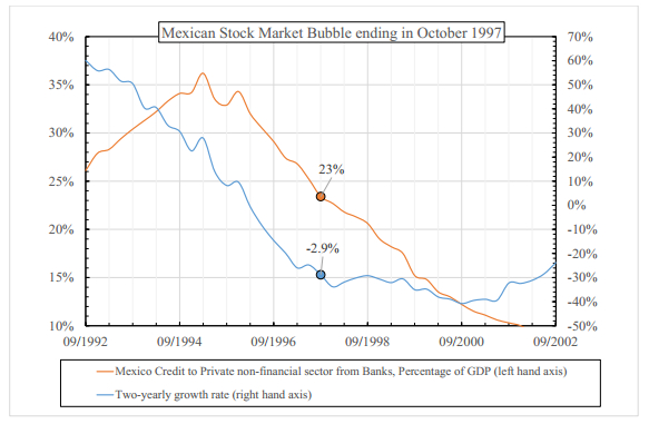
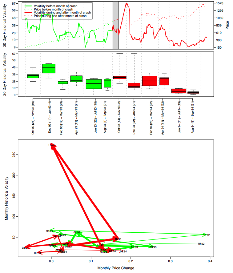
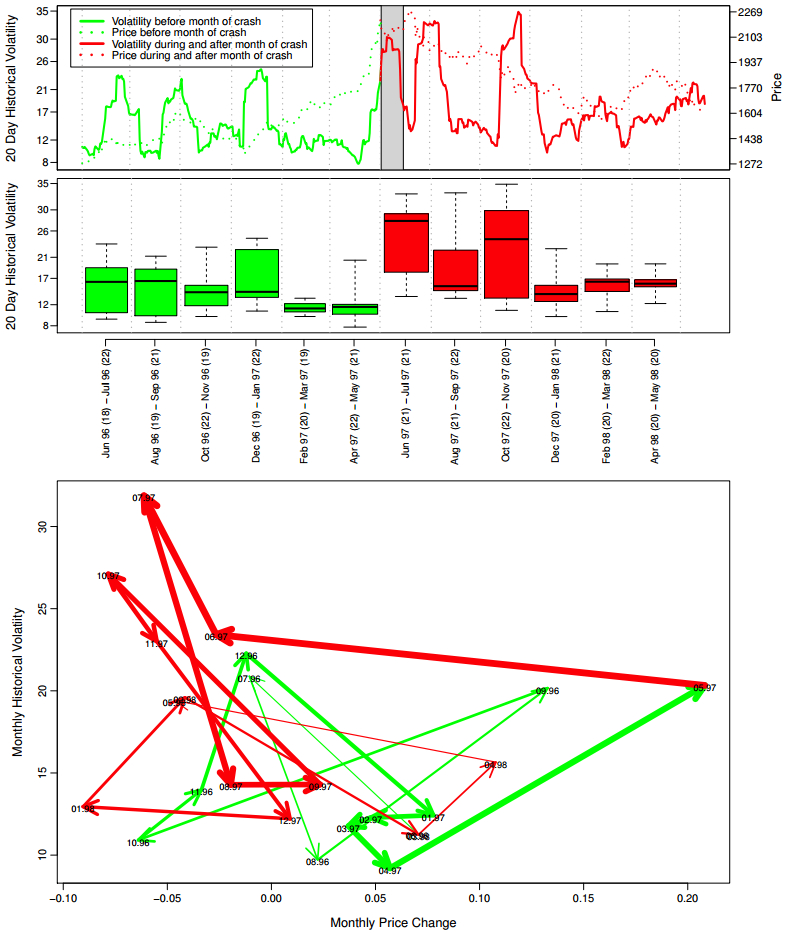
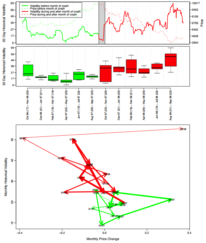
[97] | Musacchio A (2012) Mexico's Financial Crisis of 1994-1995. Technical Report 12-101, Harvard Business School Working Paper. |
[98] | Nagel S, Brunnermeier MK (2004) Hedge funds and the technology bubble. J Financ 59: 2013-2040. |
[99] | Nam CW (2008) What happened to Korea ten years ago? CESifo Forum 4: 69-73. |
[100] | Neu CR, Lowell J, Tong D (1998) Financial Crises and Contagion in Emerging Market Countries. Technical report, RAND National Security Research Division. |
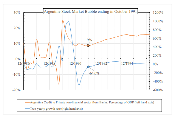
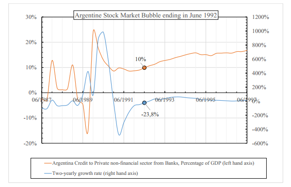
[101] | Nochteff H (1996) The Argentine experience: development or a succession of bubbles. CEPRL Rev 59: 111-126. |
[102] | Orléan A (1995) Bayesian interactions and collective dynamics of opinion -herd behavior and mimetic contagion. J Econ Behav Organ 28: 257-274. |
[103] | Perry GE, Lederman D (1998) Financial Vulnerability, Spillover Effects, and Contagion: Lessons from the Asian Crises for Latin America. Technical report, World Bank Latin American and Caribbean Studies Viewpoints. |
[104] | Phillips P, Wu Y, Yu J (2011) Explosive behavior in the 1990s Nasdaq: When did exuberance escalate asset values? Int Econ Rev 201: 201-226. |
[105] | Phillips PCB, Shi SP, Yu J (2013) Testing for multiple bubbles: Historical Episodes of Exuberance and Collapse in the S & P 500. Int Econ Rev 56: 1043-1078. |
[106] | Pinto B, Ulatov S (2010) Financial globalization and the russian crisis of 1998. The World Bank, Europe and Central Asia Region & The Managing Director? Office, Policy Research Working Paper 5312: 1-39. |
[107] | Darst DM (2013) Portfolio Investment Opportunities in Precious Metals. Jpn J Pediatr Dent 40: 32-45. |
[108] | Protter P (2013) A mathematical theory of financial bubbles. Lect Notes Math 2081: 1-108. |
[109] | Rangel GJ, Pillay SS (2007) Evidence of bubbles in the Malaysian stock market. In Asia-Pac Financ Mark: Integr, Innov Chall. |
[110] | Sang WK, Rogers JH (1995) International stock price spillovers and market liberalization: evidence from korea, japan and the united states. Int Financ Discuss Papers 2: 117-133. |
[111] | Sato K (1995) Bubbles in Japan's Stock Market: A Macroeconomic Analysis. Jpn Econ 23: 32-58. |
[112] | Scheffer M, Carpenter SR, Lenton TM, et al. (2012) Anticipating critical transitions. Science 338: 344-348. |
[113] | Scheinkman JA, Xiong W (2003) Overconfidence and speculative bubbles. J Polit Econ 111: 1183-1219. |
[114] | Scherbina A, Schlusche B (2014) Asset price bubbles: a survey. Quant Financ 14: 589-604. |
[115] | Shiller R (1979) The volatility of long term interest rates and expectations models of the term structure. J Polit Econ 87: 1190-1209. |
[116] | Shiller R (1981) Do stock prices move too much to be justified by subsequent changes in dividends? Am Econ Rev 71: 421-436. |
[117] | Shiller RJ (2006) Irrational exuberance. Crown Business, 2nd edition. |
[118] | Shiller RJ (2014) Speculative Asset Prices. Am Econ Rev 104: 1486-1517. |
[119] | Shu-jie Y, Dan L (2008) Chinese Stock Market Bubble: Inevitable or Accidental? J Xi'an Jiaotong University(Soc Sci) 6. |
[120] | Sornette D (2000) Stock Market Speculation: Spontaneous Symmetry Breaking of Economic Valuation. Phys A 284: 355-375. |
[121] | Sornette D (2004) Critical Phenomena in Natural Sciences (Chaos, Fractals, Self-organization and Disorder: Concepts and Tools). Springer 37: 9604-9605. |
[122] | Sornette D (2007) Keynote address on why stock markets crash?. Thurday 18 October 2007 at the Drobny global conference, Stockholm, Sweden, October 18-20. |
[123] | Sornette D (2017) Why Stock Markets Crash: Critical Events in Complex Financial Systems. Princeton University Press (new print with new preface). |
[124] | Sornette D, Andersen JV (2002) A nonlinear super-exponential rational model of speculative financial bubbles. Int J Mod Phys C 13: 171-188. |
[125] | Sornette D, Cauwels P (2014) 1980-2008: The Illusion of the Perpetual Money Machine and what it bodes for the future. Risks 2: 103-131. |
[126] | Sornette D, Cauwels P (2015a) Managing risk in a creepy world. J Risk Manage Financ Inst 83-108. |
[127] | Sornette D, Cauwels P (2015b) Financial bubbles: mechanisms and diagnostics. Rev Behav Econ 2: 279-305. |
[128] | Sornette D, Demos G, Zhang Q, et al. (2015) Real-time prediction and post-mortem analysis of the shanghai 2015 stock market bubble and crash. J Invest Strateg 4: 77-95. |
[129] | Sornette D, Johansen A (2001) Significance of log-periodic precursors to financial crashes. Quant Financ 1: 452-471. |
[130] | Sornette D, Johansen A, Bouchaud JP (1996) Stock market crashes, precursors and replicas. J Phys I France 6: 167-175. |
[131] | Sornette D, von der Becke S. Crashes and high frequency trading (an evaluation of risks posed by high-speed algorithmic trading). report for the UK Government project entitled "The Future of Computer Trading in Financial Markets", Foresight Driver Review -DR7, Government Office for Science, 2nd Floor, 1 Victoria Street, London SW1H 0ET, United Kingdom, 2011 (http://ssrn.com/abstract=1976249). |
[132] | Sornette D, Woodard R, Fedorovsky M (2011) The Financial Bubble Experiment: Advanced Diagnostics and Forecasts of Bubble Terminations Volume Ⅲ-Master Document. Available from: http://arXiv.org/abs/1011.2882. |
[133] | Sornette D, Woodard R, Fedorovsky M, et al. (2009) The Financial Bubble Experiment: Advanced Diagnostics and Forecasts of Bubble Terminations Volume Ⅱ -Assets Document. URL http://arXiv.org/abs/0911.0454. |
[134] | Sornette D, Zhou W-X (2002) The us 2000-2002 market descent: How much longer and deeper? Quant Financ, 2: 468-481. |
[135] | Sornette D, ZhouW-X (2004a) Evidence of fueling of the 2000 new economy bubble by foreign capital inflow: Implications for the future of the US economy and its stock market, . Phys A 332: 412-440. |
[136] | Sornette D, Zhou W-X (2004b) Causal Slaving of the U.S. Treasury Bond Yield Antibubble by the Stock Market Antibubble of August 2000. Phys A 337: 586-608. |
[137] | Sornette D, Woodard R, Zhou W-X (2009b) The 2006-2008 Oil Bubble and Beyond. Physica A 388: 1571-1576. |
[138] | Stiglitz JE (1990) Symposium on bubbles. J Econ Perspect 4: 13-18. |
[139] | Taipalus K (2012) Detecting asset price bubbles with time-series methods. Scientific monograph E 47, Helsinski. |
[140] | The Closure and Subsequent Events. a. Available from: http://www.fstb.gov.hk/fsb/ppr/report/doc/DAVISON_E_APPENDIX.PDF. |
[141] | The Gold Bubble. Available from: https://www.wealthmanagementinsights.com/userdocs/pubs/\QMU_The_Gold_Bubble__IMT_FINAL_8.15.11_TAGGED.pdf. |
[142] | The observer, consumers go sour on the market's sugar rush, 2010. Available from: http://www.guardian.co.uk/business/2010/jan/31/sugar-prices-commodities. |
[143] | Topol R (1991) Bubbles and volatility of stock prices: Effect of mimetic contagion. Econ J 101: 786-800. |
[144] | Norden SV (1996) Regime switching as a test for exchange rate bubbles. J Appl Economet 11: 219-251. |
[145] | Norden SV, Vigfusson R (1998) Avoiding the pitfalls: can regime-switching tests reliably detect bubbles? Stud Nonlinear Dyn E 2: 1-22. |
[146] | Vogel HL, Werner RA (2015) An analytical review of volatility metrics for bubbles and crashes. Int Rev Financ Anal 38: 15-28. |
[147] | Werner R (2005) The New Paradigm in Macroeconomics: Solving the Riddle of Japanese Macroeconomic Performance. Palgrave McMillan. |
[148] | West K (1987) A specification test for speculative bubbles. Q J Econ 102: 553-580. |
[149] | West K (1998) Bubbles, fads and stock price volatility tests: a partial evaluation. J Financ 43: 639-656. |
[150] | Wu Y (1997) Rational bubbles in the stock market: accounting for the U.S. stock price volatility. Econ Inq 35: 309-319. |
[151] | Xiong W(2013) Bubbles, Crises, and Heterogeneous Beliefs Handbook on Systemic Risk, Cambridge University Press 663-713. |
[152] | Yang J, Bessler DA (2008) Contagion around the October 1987 stock market crash. Eur J Oper Res 184: 291-310. |
[153] | Yao S, Luo D (2009) The Economic Psychology of Stock Market Bubbles in China. World Econ 32. |
[154] | Zhang Q, Sornette D, Balcilar M, et al. (2016) LPPLS Bubble Indicators over Two Centuries of the S & P 500 Index. Physica A 458: 126-139. |
[155] | Zhou WX, Sornette D (2003) The US2000-2003 market descent: Clarifications. Quantitative Financ 3: C39-C41. |
[156] | Zweig J (2010) Back to the future: lessons from the forgoten 'flash crash' of 1962. Intell Invest. |
1. | Anthony Carpenter, James A. Lawrence, Richard Ghail, Philippa J. Mason, The Development of Copper Clad Laminate Horn Antennas for Drone Interferometric Synthetic Aperture Radar, 2023, 7, 2504-446X, 215, 10.3390/drones7030215 | |
2. | Anupam Kr. Yadav, Suman Lata, Sandeep Kr. Singh, Arvind Kr. Singh, Tripurari Sharan, M. Z. A. Yahya, Investigating the |S11| Parameter of CPW-Fed Antennas for WiMAX and WLAN Applications, 2023, 0361-5235, 10.1007/s11664-023-10361-6 | |
3. | Anupam Kr. Yadav, Suman Lata, Sandeep Kr. Singh, Arvind Kr. Singh, Tripurari Sharan, M. N. Masri, Design and Analysis of CPW-Fed Antenna for Quad-Band Wireless Applications, 2023, 52, 0361-5235, 4388, 10.1007/s11664-023-10413-x | |
4. | Rashmi Behera, Poorna Nageswar Rao M, Suma S Lonkadi, Ajay Andhiwal, Kamaljeet Singh, 2024, Effect of Dielectric Constant Variation of High Purity Alumina Substrate on RF Performance, 979-8-3503-1755-8, 1, 10.1109/ICICACS60521.2024.10498891 | |
5. | Ngum Breayon Kwe, Vishal Yadav, Manish Kumar, Serguei V. Savilov, M. Z. A. Yahya, Sandeep Kumar Singh, A comparative study of dielectric substrate materials effects on the performance of microstrip patch antenna for 5G/6G application, 2024, 35, 0957-4522, 10.1007/s10854-024-13380-z | |
6. | Anupam Kr. Yadav, Suman Lata, Sandeep Kr. Singh, Design and Investigation of a Double-Damru (Pellet Drum)-Shaped CPW-Fed Microstrip Patch Antenna for 5G Wireless Communications, 2023, 52, 0361-5235, 4400, 10.1007/s11664-023-10414-w | |
7. | Yamiko Daniel Banda, Anupam Kumar Yadav, Sandeep Kumar Singh, Tripurari Saran, Serguei V. Savilov, M.Z.A. Yahya, Fiberglass Interwoven Substrate Laminated Penta‐Band Microstrip Antenna, 2025, 414, 1022-1360, 10.1002/masy.202400162 |
Antennas | Schematic Configuration of Proposed Antennas (Units: mm) | |||||||||
Ground Terminal-1 (T1) | Ground Terminal-2 (T2) | Ground Terminal-3 (T3) | Antenna Response | |||||||
Lx(T1) | Ly(T1) | t(T1) | Lx(T2) | Ly(T2) | t(T2) | Lx(T3) | Ly(T3) | t(T3) | ||
Base Ant. [17] | 24.0 | 18 | 0.4 | 24.0 | 14 | 0.4 | NA | NA | NA | Single-band |
Base Ant. [18] | 21.5 | 14.7 | 4.2 | 21.5 | 14.7 | 4.2 | NA | NA | NA | Single-band |
Proposed Ant.1 | 20.5 | 19 | 0.5 | 20.5 | 15 | 0.5 | 05 | NA | 0.5 | Dual-band |
Proposed Ant.2 (T) | 20.5 | 19 | 0.5 | 20.5 | 15 | 0.5 | 07 | 8 | 0.5 | Triple-band |
Proposed Ant.2 (Q) | 20.5 | 19 | 0.5 | 20.5 | 15 | 0.5 | 07 | 16 | 0.5 | Triple/Quad band |
Lx: Length in x-direction: Ly: Length in y-direction: Lx(T1): Length of terminal-1 in x-direction; Lx(T2): Length of terminal-2 in x-direction; Lx(T3): Length of terminal-3 in x-direction; Ly(T1): Length of terminal-1 in y-direction; Ly(T2): Length of terminal-2 in y-direction; Ly(T3): Length of terminal-3 in y-direction; t(T1): Width thickness of terminal-1; t(T2): Width thickness of terminal-2; t(T3): Width thickness of terminal-3; (T): Triple-band; (Q): Quad-band; NA: Not Applicable |
Property | Rogers | Arlon | FR4 | Alumina | Condition/Range |
Dielectric Constant (εr) | 2.2 | 3.2 | 4.3 | 9.8 | 1 to 10 GHz |
Dissipation Factor (tan𝛿) | 0.0004 | 0.0038 | 0.017 | 0.0020 | 10 GHz |
Thermal Coefficient of εr (ppm/°K) | −125 | −110 | −80 | −43 | −55 to +125℃ |
Thermal Conductivity (W/m.K) | 0.26 | 0.235 | 0.45 | 0.76 | 80 to 100℃ |
Specific Heat (J/g.K) | 0.96 | 0.90 | 0.95 | 0.72 | - |
Volume Resistivity (MΩ-cm) | 2x10⁷ | 1.2x10⁹ | 8x10⁷ | 2x10⁸ | - |
Surface Resistivity (MΩ) | 3x10⁷ | 4.5x10⁷ | 2x10⁵ | 4x10⁷ | - |
Break down voltage (kV) | > 60 | > 45 | > 32 | > 18 | - |
Moisture Absorption (%) | 0.02 | 0.06 | 0.25 | 0.16 | - |
Design Steps of Ant.1 | Various Length of Ground Terminal Stubs and Substrate Thickness (t) | Resonance Frequencies (frN), (N = 1, 2) | ||||||||
Lx(T1) (mm) | Ly(T1) (mm) | Lx(T2) (mm) | Ly(T2) (mm) | Lx(T3) (mm) | FR4 (t) (mm) | fr1 (GHz) | |S11|1 (−dB) | fr2 (GHz) | |S11|2 (−dB) | |
Step-1 | - | - | - | - | 4 | 0.76 | 2.90 | 20 | - | - |
- | - | - | - | 5 | 0.76 | 2.90 | 21 | - | - | |
- | - | - | - | 6 | 0.76 | 2.85 | 22 | - | - | |
- | - | - | - | 7 | 0.76 | 2.85 | 23 | - | - | |
- | - | - | - | 8 | 0.76 | 2.80 | 23 | - | - | |
Step-2 | 18.50 | 19 | - | - | 7 | 0.76 | 1.90 | 20 | 2.85 | 34 |
19.50 | 19 | - | - | 7 | 0.76 | 1.75 | 20 | 2.85 | 34 | |
20.50 | 19 | - | - | 7 | 0.76 | 1.90 | 20 | 2.85 | 34 | |
21.50 | 19 | - | - | 7 | 0.76 | 1.75 | 23 | 2.80 | 35 | |
22.50 | 19 | - | - | 7 | 0.76 | 1.80 | 23 | 2.80 | 36 | |
Step-3 | - | - | 18.50 | 15.25 | 7 | 0.76 | 1.40 | 16 | 2.75 | 29 |
- | - | 19.50 | 15.25 | 7 | 0.76 | 1.35 | 19 | 2.75 | 30 | |
- | - | 20.50 | 15.25 | 7 | 0.76 | 1.35 | 19 | 2.75 | 39 | |
- | - | 21.50 | 15.25 | 7 | 0.76 | 1.35 | 20 | 2.75 | 39 | |
- | - | 22.50 | 15.25 | 7 | 0.76 | 1.40 | 22 | 2.75 | 39 | |
Step-4 | 20.50 | 19 | 20.50 | 15 | 1 | 0.76 | 2.10 | 45 | 2.85 | 30 |
20.50 | 19 | 20.50 | 15 | 3 | 0.76 | 2.10 | 55 | 2.85 | 30 | |
20.50 | 19 | 20.50 | 15 | 5 | 0.76 | 2.05 | 40 | 2.80 | 32 | |
20.50 | 19 | 20.50 | 15 | 7 | 0.76 | 1.90 | 30 | 2.75 | 45 |
Design Steps of Ant.2 | Various Length of Ground Terminal Stubs | frN in GHz at (−dB); N = 1, 2, 3 | |||||||
Lx(T1) (mm) | Ly(T1) (mm) | Lx(T2) (mm) | Ly(T2) (mm) | Lx(T3) (mm) | Ly(T3) (mm) | fr1 at (−dB) | fr2 at (−dB) | fr3 at (−dB) | |
Step-1 | 20.50 | 19 | 20.50 | 15 | 1 | 8 | 1.25 (12) | 1.80 (25) | 2.7 (36) |
Step-2 | 20.50 | 19 | 20.50 | 15 | 3 | 12 | 1.75 (25) | 2.65 (31) | - |
Step-3 | 20.50 | 19 | 20.50 | 15 | 5 | 16 | 1.70 (24) | 2.65 (28) | 3.5 (14) |
Step-4 | 20.50 | 19 | 20.50 | 15 | 7 | 20 | 1.65 (20) | 2.60 (25) | 3.2 (16) |
|S11| parameter of Ant.1 shown in Figure | Substrate Material (εr) | Substrate Thickness (t) (mm) | Stub Lx(T3) (mm) | Resonance Frequency (GHz) | IBW S11≤ −20 dB (GHz) | IBW S11≤ −10 dB (GHz) | ||
fr1 | fr2 | (IBW)1 | (IBW)2 | (IBW)Total | ||||
Figure 12(a) | Alumina (9.9) | 0.51 | 5 | 1.90 | 2.80 | 0.20 | 0.50 | 2.0 |
Figure 12(b) | FR4 (4.3) | 0.76 | 5 | 2.05 | 2.80 | 0.25 | 0.50 | 2.0 |
Figure 12(c) | Arlon (3.2) | 0.95 | 5 | 2.10 | 2.95 | 0.25 | 0.50 | 2.1 |
Figure 12(d) | Rogers (2.2) | 1.11 | 5 | 2.20 | 3.40 | 0.15 | 0.55 | 2.5 |
|S11| parameter of Ant.2 | Substrate Material (εr) | Substrate Thickness (mm) | Stub Ly(T3) (mm) | frN in GHz (N = 1, 2, 3, 4) | IBW in GHz at (−dB) | ||||||
fr1 | fr2 | fr3 | fr4 | (IBW)1 | (IBW)2 | (IBW)3 | (IBW)4 | ||||
Figure 13(a) | Rogers (2.2) | 0.76 | 8 | 1.45 | 2.10 | 3.35 | - | 0.25 (10) | 0.35 (15) | 0.50 (20) | - - |
Arlon (3.2) | 1.90 | 3.00 | - | - | 0.40 (15) | 0.50 (20) | - - | - - | |||
FR4 (4.3) | 1.30 | 1.80 | 2.65 | - | 0.15 (10) | 0.45 (15) | 0.50 (20) | - - | |||
Alumina (9.9) | 1.50 | 2.00 | - | - | 0.17 (20) | 0.45 (20) | - - | - - | |||
Figure 13(b) | Rogers (2.2) | 0.76 | 16 | 1.40 | 1.90 | 3.20 | 3.85 | 0.10 (10) | 0.45 (12) | 0.75 (15) | 0.30 (20) |
Arlon (3.2) | 1.80 | 2.75 | 3.65 | - | 0.35 (13) | 1.00 (15) | 0.50 (10) | - - | |||
FR4 (4.3) | 1.75 | 2.65 | 3.50 | - | 0.25 (15) | 0.40 (20) | 0.25 (10) | - - | |||
Alumina (9.9) | 1.40 | 1.90 | - | - | 0.10 (20) | 0.45 (20) | - - | - - |
|S11| parameter of Ant.2 shown in Figure | Substrate Material (εr) | Substrate Thickness (t, mm) | frN in GHz, (N = 1, 2, 3, 4) | |||
fr1 | fr2 | fr3 | fr4 | |||
Figure 14(a) | Rogers (2.2) | 0.95 | 1.40 | 1.90 | 3.20 | 3.85 |
1.11 | 1.35 | 1.90 | 3.10 | 3.80 | ||
1.35 | - | 1.85 | 3.10 | 3.75 | ||
1.50 | - | 1.85 | 3.05 | 3.75 | ||
Figure 14(b) | Arlon (3.2) | 0.76 | 1.80 | 2.90 | 3.75 | - |
0.95 | 1.78 | 2.90 | 3.70 | - | ||
1.11 | 1.75 | 2.77 | 3.55 | - | ||
1.35 | 1.65 | 2.75 | 3.50 | - | ||
Figure 14(c) | FR4 (4.3) | 0.51 | 1.85 | 3.15 | 3.80 | - |
0.63 | 1.80 | 2.90 | 3.65 | - | ||
0.76 | 1.75 | 2.65 | 3.50 | - | ||
0.95 | 1.65 | 2.45 | 3.40 | - | ||
Figure 14(d) | Alumina (9.9) | 0.31 | - | 3.25 | 4.10 | - |
0.40 | 1.90 | 3.20 | 3.95 | - | ||
0.51 | 1.60 | 2.65 | 3.35 | - | ||
0.76 | 1.402 | 1.95 | - | - |
Resonance Frequencies (fr) of Proposed Ant.1 and Ant.2 | ||||||||||
Laminated Antenna (εr) | Proposed Ant.1 | Proposed Ant.2 | ||||||||
t (mm) | fr1 (GHz) | fr2 (GHz) | Response | t (mm) | fr1 (GHz) | fr2 (GHz) | fr3 (GHz) | fr4 (GHz) | Response | |
Rogers (2.2) | 1.11 | 2.15 | 3.40 | Dual-band | 0.95 | 1.40 | 1.90 | 3.20 | 3.80 | Quad-band |
Arlon (3.2) | 0.95 | 2.10 | 2.90 | Dual-band | 0.76 | - | 1.80 | 2.85 | 3.65 | Triple-band |
FR4 (4.3) | 0.76 | 2.05 | 2.80 | Dual-band | 0.51 | - | 1.80 | 3.10 | 3.75 | Triple-band |
Alumina (9.9) | 0.51 | 1.90 | 2.80 | Dual-band | 0.40 | - | 1.85 | 3.15 | 3.95 | Triple-band |
[Ref.] Year | Substrate Material | Size (mm2) | frN in GHz (N=1, 2, 3, 4) | IBW in GHz at ≤ −10 dB | |||||||
(εr) | t (mm) | fr1 | fr2 | fr3 | fr4 | (IBW1)-dB | (IBW2)-dB | (IBW3)-dB | (IBW4)-dB | ||
[06] 2006 | FR4 (4.4) | 0.80 | 120×40 | 2.45 | 5.45 | - | - | (0.51)−10 dB | (1.01)−10 dB | - | - |
[07] 2010 | Rogers (2.2) | 2.00 | 64×62 | 2.44 | 3.55 | - | - | (0.11)−10 dB | (0.14)−10 dB | (0.63)−10 dB | - |
[08] 2015 | Rogers (2.33) | 3.20 | 40×28 | 2.45 | 3.50 | 5.28 | - | (0.14)−10 dB | (0.15)−10 dB | (0.24)−10 dB | - |
[09] 2018 | FR4 (4.2) | 1.60 | 70×70 | 2.31 | 2.40 | 2.48 | - | (0.05)−10 dB | (0.06)−10 dB | (0.06)−10 dB | - |
[10] 2019 | FR4 (4.2) | 0.80 | 30×28 | 2.62 | 3.55 | 5.56 | - | (0.25)−10 dB | (0.48)−10 dB | (0.50)−20 dB | - |
[11] 2019 | FR4 (4.4) | 1.60 | 65×30 | 2.45 | 5.15 | - | - | (0.45)−10 dB | (0.45)−10 dB | - | |
[12] 2020 | FR4 (4.3) | 1.60 | 50×50 | 2.45 | 3.80 | 5.80 | - | (0.08)−10 dB | (0.95)−20 dB | (1.20)−20dB | - |
[13] 2020 | Rogers (10.2) | 1.27 | 25×31 | 2.46 | 5.11 | - | - | (0.11)−10 dB | (0.07)−10 dB | - | - |
[14] 2021 | Rogers (3.0) | 0.80 | 40×60 | 1.64 | 1.79 | 2.11 | 2.43 | (0.04)−10 dB | (0.10)−10 dB | (0.07)−10 dB | (0.08)−10dB |
Duroid (2.2) | 1.60 | 1.75 | 1.87 | 2.24 | - | (0.07)−5 dB | (0.06)−5 dB | (0.05)−5 dB | - | ||
FR4 (4.4) | 1.60 | 1.63 | 1.80 | 2.31 | - | (0.11)−10 dB | (0.09)−10 dB | (0.07)−10 dB | - | ||
[15] 2021 | FR4 (4.4) | 0.80 | 50×50 | 2.50 | 3.60 | 6.00 | - | (0.20)−16 dB | (0.90)−20 dB | (0.30)−20 dB | - |
[16] 2021 | FR4 (4.4) | 1.60 | 116×116 | 1.02 | 1.75 | - | - | (0.35)−15 dB | (0.38)−12 dB | - | - |
Proposed Ant.1 | Rogers (2.2) | 1.11 | 50×50 | 2.15 | 3.40 | - | - | (0.70)−10 dB | (0.75)−10 dB | - | - |
Arlon (3.2) | 0.95 | 2.10 | 2.90 | - | - | (0.40)−10 dB | (0.55)−20 dB | - | - | ||
FR4 (4.3) | 0.76 | 2.05 | 2.80 | - | - | (0.45)−10 dB | (0.50)−20 dB | - | - | ||
Alumina (9.9) | 0.51 | 1.90 | 2.80 | - | - | (0.55)−15 dB | (0.60)−20 dB | - | - | ||
Proposed Ant.2 | Rogers (2.2) | 0.95 | 50×50 | 1.40 | 1.90 | 3.20 | 3.80 | (0.25)−10 dB | (0.50)−12 dB | (0.75)−15 dB | (0.55)−15dB |
FR4 (4.3) | 0.51 | - | 1.80 | 3.10 | 3.75 | - | (0.35)−12 dB | (0.70)−15 dB | (0.65)−10dB |