Loading [MathJax]/jax/element/mml/optable/GeneralPunctuation.js
Research article Special Issues

An optimal scheme to boost immunity and suppress viruses for HIV by combining a phased immunotherapy with the sustaining antiviral therapy

  • Despite many approaches to treat HIV virus, the endeavor, due to the inability of therapy to eradicate HIV infection, has been aroused to formulate rational therapeutic strategies to establish sustained immunity to suppress viruses after stopping therapy. In this paper, incorporating the time lag of the expansion of immune cells, we propose an explicit model with continuous antiretroviral therapy (CATT) and an intermittent immunotherapy to describe an interaction of uninfected cells, HIV virus and immune response. Two kinds of bistability and the sensitivities of the amplitude and period of the periodic solution with respect to all of parameters indicate that both ε and b relating to the therapy are scheduled to propose an optimal treatment tactics. Furthermore, taking a patient performed a CATT but with an unsuccessful outcome as a example, we inset a phased immunotherapy into the above CATT and then adjust the therapeutic session as well as the inlaid time to quest the preferable therapeutic regimen. Mathematically, we alter the solution of system from the basin of the attraction of the immune-free equilibrium to the immune control balance when the treatment is ceased, meanwhile minimize the cost function through a period of combined therapy. Due to the particularity of our optimal problem, we contribute a novel optimization approach by meshing a special domain on the antiretroviral and immunotherapy parameters ε and b, to catch an optimal combined treatment scheme. Simulations exhibit that early mediating immunotherapy suppresses the load of virus lower while shortening the combined treatment session does not reduce but magnify the cost function. Our results can provide some insights into the design of optimal therapeutic strategies to boost sustained immunity to quell viruses.

    Citation: Youyi Yang, Yongzhen Pei, Xiyin Liang, Yunfei Lv. An optimal scheme to boost immunity and suppress viruses for HIV by combining a phased immunotherapy with the sustaining antiviral therapy[J]. Mathematical Biosciences and Engineering, 2020, 17(5): 4578-4608. doi: 10.3934/mbe.2020253

    Related Papers:

    [1] B. M. Adams, H. T. Banks, Hee-Dae Kwon, Hien T. Tran . Dynamic Multidrug Therapies for HIV: Optimal and STI Control Approaches. Mathematical Biosciences and Engineering, 2004, 1(2): 223-241. doi: 10.3934/mbe.2004.1.223
    [2] Divya Thakur, Belinda Marchand . Hybrid optimal control for HIV multi-drug therapies: A finite set control transcription approach. Mathematical Biosciences and Engineering, 2012, 9(4): 899-914. doi: 10.3934/mbe.2012.9.899
    [3] Seyedeh N. Khatami, Chaitra Gopalappa . A reinforcement learning model to inform optimal decision paths for HIV elimination. Mathematical Biosciences and Engineering, 2021, 18(6): 7666-7684. doi: 10.3934/mbe.2021380
    [4] Prathibha Ambegoda, Hsiu-Chuan Wei, Sophia R-J Jang . The role of immune cells in resistance to oncolytic viral therapy. Mathematical Biosciences and Engineering, 2024, 21(5): 5900-5946. doi: 10.3934/mbe.2024261
    [5] Sophia Y. Rong, Ting Guo, J. Tyler Smith, Xia Wang . The role of cell-to-cell transmission in HIV infection: insights from a mathematical modeling approach. Mathematical Biosciences and Engineering, 2023, 20(7): 12093-12117. doi: 10.3934/mbe.2023538
    [6] Joseph Malinzi, Rachid Ouifki, Amina Eladdadi, Delfim F. M. Torres, K. A. Jane White . Enhancement of chemotherapy using oncolytic virotherapy: Mathematical and optimal control analysis. Mathematical Biosciences and Engineering, 2018, 15(6): 1435-1463. doi: 10.3934/mbe.2018066
    [7] Gesham Magombedze, Winston Garira, Eddie Mwenje . Modelling the immunopathogenesis of HIV-1 infection and the effect of multidrug therapy: The role of fusion inhibitors in HAART. Mathematical Biosciences and Engineering, 2008, 5(3): 485-504. doi: 10.3934/mbe.2008.5.485
    [8] Damilola Olabode, Libin Rong, Xueying Wang . Stochastic investigation of HIV infection and the emergence of drug resistance. Mathematical Biosciences and Engineering, 2022, 19(2): 1174-1194. doi: 10.3934/mbe.2022054
    [9] Tinevimbo Shiri, Winston Garira, Senelani D. Musekwa . A two-strain HIV-1 mathematical model to assess the effects of chemotherapy on disease parameters. Mathematical Biosciences and Engineering, 2005, 2(4): 811-832. doi: 10.3934/mbe.2005.2.811
    [10] Cameron Browne . Immune response in virus model structured by cell infection-age. Mathematical Biosciences and Engineering, 2016, 13(5): 887-909. doi: 10.3934/mbe.2016022
  • Despite many approaches to treat HIV virus, the endeavor, due to the inability of therapy to eradicate HIV infection, has been aroused to formulate rational therapeutic strategies to establish sustained immunity to suppress viruses after stopping therapy. In this paper, incorporating the time lag of the expansion of immune cells, we propose an explicit model with continuous antiretroviral therapy (CATT) and an intermittent immunotherapy to describe an interaction of uninfected cells, HIV virus and immune response. Two kinds of bistability and the sensitivities of the amplitude and period of the periodic solution with respect to all of parameters indicate that both ε and b relating to the therapy are scheduled to propose an optimal treatment tactics. Furthermore, taking a patient performed a CATT but with an unsuccessful outcome as a example, we inset a phased immunotherapy into the above CATT and then adjust the therapeutic session as well as the inlaid time to quest the preferable therapeutic regimen. Mathematically, we alter the solution of system from the basin of the attraction of the immune-free equilibrium to the immune control balance when the treatment is ceased, meanwhile minimize the cost function through a period of combined therapy. Due to the particularity of our optimal problem, we contribute a novel optimization approach by meshing a special domain on the antiretroviral and immunotherapy parameters ε and b, to catch an optimal combined treatment scheme. Simulations exhibit that early mediating immunotherapy suppresses the load of virus lower while shortening the combined treatment session does not reduce but magnify the cost function. Our results can provide some insights into the design of optimal therapeutic strategies to boost sustained immunity to quell viruses.


    Human immunodeficiency virus (HIV) and HIV treatment have always received extensive attention by many researchers. In 1996, Dr. He invented the famous 'cocktail' therapy, namely highly active antiretroviral therapy (HAART), from which AIDS has changed from an 'incurable disease' to a controllable 'chronic disease' [1]. Since then, more attention has been paid to antiviral drug therapies which aim to boost virus-specific immune response by resisting or destroying viral infections [2,3,4,5,6]. Hence, HAART can effectively control viral replication in patients for a long time, and patients can even live to their life expectancy. However HAART has some limitations, for instance, HIV is not completely eradicated, and the virus remains hidden in some immune cells, returning once the patient has stopped taking the antiviral; life-long HAART is thus required [7], which brings many inconveniences and various side effects. Therefore, numerous HIV scientists are devoted to seeking novel cures for AIDS including immunotherapy [7,8,9,10,11] of AIDS.

    At present, the immunotherapy of AIDS has the following aspects: Anti-HIV strategy based on antibody, such as broadly neutralizing antibodies (bNabs) [8], immune checkpoint blockers (ICBs) [12] and antibody-mediated cell strategies to eliminate HIV infection [7]; Strategy of therapeutic vaccine based on HIV-1; Other immunotherapies, such as the α4β7 blocker (vedolizumab) [13], can significantly reduce the exposure of target cells to HIV by blocking the surface of CD4+ T lymphocytes α4β7 molecules to restrict the return of CD4+ cells to the intestinal mucosa; Immunotherapy combined with antiviral therapy and so on. The strategy of HIV-1 therapeutic vaccine is based on a class of HIV-infected people known as "elite controllers" [14]. Studies have found that very few infected people can "peacefully coexist" with the virus for a long time. Their immune system can naturally control the replication of the virus and avoid the damage of the virus to the immune system. "Therapeutic vaccine" aims to reactivate the immune system of the infected person through the vaccine, so that the infected person can spontaneously produce specific CD8+ T lymphocyte for HIV-1. After interruption of antiviral treatment, it can still inhibit the virus and achieve functional cure.

    It was argued that sustained virus-specific immunity for HIV infection may be established via early therapy and structured therapy interruptions [15,16]. Later, using a mathematical framework, Komarova et al. [17] show that a single phase of antiviral therapy is also possible to achieve this goal. Essentially, it is shown by [17] that a immune-free equilibrium (no sustained immunity) and an immune control equilibrium (with sustained immunity) are both stable. This bistability allows a solution from the basin of the attraction of the immune-free equilibrium to be lifted to that of the immune control equilibrium via a single phase of therapy, resulting in sustained immunity when the treatment is stopped.

    However, HIV is rapidly reproduced and quickly becomes resistant to any single drug [18,19,20,21]. A multi-institutional team of researchers, led by the Wistar Institute, has announced the results of a clinical trial that showed the immune system can engage in fighting HIV infection if given the right boost. In their studies, HIV-infected volunteers suspended their daily antiretroviral therapy to receive weekly doses of interferon-α, an antiviral chemical produced by the human immune system. Dramatically, 45 percent of these patients sustained the HIV control under the lower level. These researches provide the first clinical evidence for reducing the persistent amount of HIV in patients and increasing the ability to control HIV without continued antiretroviral therapy [22]. Hence, boosting specific immune responses by therapeutic vaccine or immune regulation with interferon is possible and promising.

    One traditional model with antiviral drug therapy, sketched the connection among uninfected cells, infected cells and virus, was proposed by Nowak et al. [23], which has been extensively and deeply probed [24,27]. Another classical model depicted the relation between virus and immune cells was used to snatch the boosting immunity by single or multiple phases of therapy [17,28,29]. But how to tangle and capture reasonably the interaction among uninfected cells, virus and immune cells is challenging. Furthermore, if combining antiviral drug with immune regulation therapy, what is the dynamic outcome of three populations? In order to sustain viral suppression and immunological motivation, which parameters and why can be adjusted to regulate therapy schemes? If we acquire these parameters, further how to optimize these parameters to boost immune responses to sustain viral suppression at the minimum cost after stopping treatment? These are significative and challenging pursuits.

    The outline is instructed as follows: In Section 2, a mathematical model is formulated. In Section 3, the well-posedness and the existence of equilibrium are explored. The stability of system (2.5) as well as Hopf bifurcation are discussed in Section 4. In Section 5, the sensitivity of the periodic solution with sustained immunity is investigated. In Section 6, combination treatment is discussed in detail. Finally, some conclusions are drawn in Section 7.

    To answer the above issues, after principally consulting [17,23,29] and other literatures, we list several main models and then formulate our model.

    Uninfected cells, infected cells, virus model and immune response model

    Viral reproduction always involves host cells and uses the cellular machinery for the synthesis of their genome and other components. Nowak et al. [30] describe the relationship between the populations of uninfected cells, x, infected cells that produce virus, y, and free virus particles, v, the abundance of virus-specific CTLs z, and design a simple but natural mathematical model based on ordinary differential equations [23,24,30]:

    dxdt=sdxβxv,dydt=βxvμypyz,dvdt=kyωv,dzdt=cyzbz.

    Uninfected cells are produced at a constant rate s and die at the rate dx. Free virus infects uninfected cells to produce infected cells at rate βxv. Infected cells die at rate μy. New virus is produced from infected cells at rate ky and dies at rate ωv. The average life-times of infected cells are thus given by 1/μ. Hence, the average number of virus particles produced over the lifetime of a single infected cell (the burst size) is given by k/μ. The rate of CTL proliferation in response to antigen is given by cyz. In the absence of stimulation, CTLs decay at rate bz. Infected cells are killed by CTLs at rate pyz.

    By the quasi steady-state assumption for the turnover of free virus is much faster than that of infected cells [25,26], we know that y=(ω/k)v at steady-state from the 3th equation of the above model, that is, the amount of free virus is simply proportional to the number of infected cells. Hence the 2nd and 4th equations of the above model are equivalent to v=kβxv/ωμvpvz and z=ωcvz/kbz, respectively. For convenience, let k/ω=ϑ. Then the above four-dimensional model is reduced to a three-dimensional one:

    dxdt=sdxβxv,dvdt=ϑβxvμvpvz,dzdt=cvz/ϑbz, (2.1)

    Virus and immune response model

    Note that the immune response after viral infection is universal and necessary to eliminate or control the disease. Antibodies, cytokines, natural killer cells, and T cells are essential components of a normal immune response to a virus. Indeed, in most viral infections, cytotoxic T lymphocytes (CTLs) play a critical role in antiviral defense by attacking virus-infected cells. It is believed that they are the main host immune factor that limit the development of viral replication in vivo and thus determine virus load [30,31,32]. Therefore, the population dynamics of viral infection with CTL response has been paid much attention in the last few decades. Komarova et al. [17] established a mathematical model to explore the relation between the virus population v and a population of immune cells z:

    dvdt=rv(1vk)avpvz,dzdt=cvz1+ηvbzmvz, (2.2)

    The virus population is assumed to grow logistically: r is the viral replication rate at low viral loads, and assume that this rate decreases linearly with increased viral load to reach zero at a viral load k. The virus population decays at a rate a. Overall, this gives a logistic growth with a net growth rate ra and a carrying capacity of k(ra)/r. Moreover, virus is killed by the CTL response at a rate pvz, corresponding to lytic effector mechanisms of CTL response. Immune cells at time t due to virus activation, expand at a rate cvz/1+ηv [33,34], which depends on the viral load and the number of immune cells at time t, and implies that when the virus load is low, the level of immune response is simply proportional to both the virus population, v, and the immune response, z, but that the immune response saturates when the virus load is sufficiently high. Immune cells die at rate b and are inhibited by the virus population at rate mvz [28].

    In addition, it has been recognized that the immune response is not instantaneous and the process involves a sequence of events such as antigenic activation, selection, and proliferation of the immune cells. It is believed that they are the main host immune factor that limit the development of viral replication in vivo and thus determine virus load [35,36]. Therefore, the time lag between these events should be taken into consideration in modeling and the relationship between virus population and a population of immune cells can be simply described as:

    dvdt=M(v)avg1(v,z),dzdt=h(v(tτ),z(tτ))bzg2(v,z), (2.3)

    The virus population grows at a rate described by the function M(v). Immune expansion is determined by the virus load and the number of immune cells z at time tτ and τ is the time lag for the production of new immune cells mediated by the infection, which is described by the function h(v(tτ),z(tτ)). Functions g1(v,z) and g2(v,z) represent the interaction between immune cells and virus and further h,g1 and g2 can be written as Holling functional response.

    Uninfected cells, virus and immune response model with combined treatment

    For the sake of deep studying the dynamic behavior of immune response in human body, tangling (2.1) with (2.3), one formulates a model consisted of three variables including uninfected target cells x, virus v, and CTL response z. Specifically, insetting a phased immunotherapy into a continuous antiviral treatment (such as reverse transcriptase inhibitors (RTIs)) [24,27,28,37], the following model with hybrid treatment comes into being:

    {dxdt=sdx(1Ψ(t))βxv,dvdt=(1Ψ(t))ϑβxvavpvz,dzdt=cv(tτ)z(tτ)1+ηv(tτ)bzmvz+Θ(t)z, (2.4)

    where

    Ψ(t)={ε0t[0,t1),εt[t1,t2],ε0t(t2,T],Θ(t)={0t[0,t1),ˉbt[t1,t2],0t(t2,T].

    Now before the detailed indagation, several symbols are given. Suppose that the patient remains on the antiviral treatment during the whole course of patient observed [0,T]. While t1(0,T) and t2(0,T) with t1<t2 are the initial and terminal time of immunotherapy respectively. Then [0,t1] and [t2,T] are called the single antiviral treatment session (ATTS), while [t1,t2] is referred to as the combined treatment session (CTS). 0ε0,ε1 describe the effectiveness of antiretroviral drugs [38] during ATTS and CTS; ˉb0 represents the efficacy of immunotherapy, which could boost specific immune responses by therapeutic vaccine or immune regulation with interferon. The biological meaning of parameters is presented in Table 1.

    Table 1.  Parameters and values used in simulations for system (2.5).
    Parameter Description Value Reff.
    s Production rate of Target cell 0.7 cells μl1 day1
    d Death rate of Target cell 0.01 day1 [43]
    k Viral production rate 90 day1 [44]
    β Infection rate of Target cell 0.045 μl virus1 day1
    ε Efficacy of antiviral drugs 0.8
    a Death rate of virus 3 day1 [29]
    p Killing rate of virus 0.3 μl cells1 day1
    by immune cells
    c Proliferation rate of immune cells 0.6 μl virus1 day1 [43]
    η Hill coefficient in the rate of 1 μl virus1 [43]
    immune cell production
    b Death rate of immune cells 0.3 day1 [45]
    m Immune impairment rate 0.05 μl virus1 day1 [45]
    τ Time lag for production of new [35]
    immune cells mediated by infection

     | Show Table
    DownLoad: CSV

    The initial conditions for system (2.4) are

    (ϕ1(θ),ϕ2(θ),ϕ3(θ))C+=C([τ,0],R3+),ϕi(0)>0,i=1,2,3,

    where R3+=(x,v,z)R3:x0,v0,z0. Therefore, all the standard results on existence, uniqueness and continuous dependence on initial condition of solutions are evidently satisfied.

    Due to the inability of single antiviral therapy to eradicate HIV infection for many patients, in this paper we devote to the therapeutic effect of the intermittent immunotherapy based on a continuous antiviral treatment. So we firstly aim at the dynamic behaviors of following model which is the case in model (2.4) under Ψε and Θ(t)0:

    {dxdt=sdx(1ε)βxv,dvdt=(1ε)ϑβxvavpvz,dzdt=cv(tτ)z(tτ)1+ηv(tτ)bzmvz. (2.5)

    For the nonnegativeness and boundedness of solutions, we state the following lemma.

    Lemma 3.1. There exists a positively invariant box Ω=[(x,v,z)R3+:0xMϑ,0vM,0zcpM] in R3+ such that all solutions of (2.5) with nonnegative initial conditions approach Ω as t, where M=sϑμ+κ, μ=min{a,b,d} and κ is a positive constant.

    Proof. Solving v(t) in the second equation of (2.5) yields

    v(t)=v(0)et0[(1ε)ϑβx(θ)apz(θ)]dθ,fort0.

    Next we show that x(t) is nonnegative for t>0. Assume to the contrary that x(t)0 for t[0,ˆt) and x(ˆt)=0 with x(ˆt)<0 for some ˆt>0. Then it follows from the first equation of system (2.5) that x(ˆt)=s>0. This is a contradiction. Thus x(t)0 for all t0. Similarly, we can obtain that z(t) is nonnegative for t>0.

    Adding up the three equations of (2.5), one gets

    (ϑx(t)+v(t)+pcz(t+τ))sϑdϑx(t)av(t)pv(t)z(t)+pv(t)z(t)1+ηv(t)pcbz(t+τ)sϑμ(ϑx(t)+v(t)+pcz(t+τ)),

    where μ=min{a,b,d}. By the comparison theorem, we obtain that limt(ϑx(t)+v(t)+pcz(t+τ))sϑμ. That is, for a positive constant κ,ϑx(t)+v(t)+pcz(t)sϑμ+κ˙=M holds for τ=0 and t large enough. Then we get a positively invariant box Ω={(x,v,z)R3+:0xMϑ,0vM,0zcpM} in R3+ by the non-negativity of x(t),v(t) and z(t), such that all solutions with nonnegative initial conditions approach as t.

    Next, we consider the existence of equilibrium by the right side of system (2.5).

    Virus-free equilibrium

    Clearly, system (2.5) admits a virus-free equilibrium E0=(x0,0,0), corresponding to the maximal level of healthy CD4+T cells and the extinction of free virus, where x0=s/d.

    Virus-boom and immune-free equilibrium

    When z=0, we solve the first two equation of the right side of (2.5) obtains a virus-boom and immune-free equilibrium E1(x1,v1,0), corresponding to partial CD4+T cells are infected but no CTL response, where

    x1=a(1ε)ϑβ,v1=sϑad(1ε)β=dϑ((1ε)ϑβsad1)ax1.

    This implies that the level of the virus depends on related parameters of uninfected cells and the virus. In addition, we know that if (1ε)ϑβs/(ad)>1, then system (2.5) has a virus-boom and immune-free equilibrium and the virus load in direct proportion to the population of uninfected cells at E1. At this time, there is a linear relationship between the virus and the uninfected cells because of the disappearance of immune response.

    Virus-suppression and immune-boost equilibrium

    In the case of z0, corresponding to CTL response, assume that the Ei(xi,vi,zi)(i=1,2) is a virus-suppression and immune-boost equilibrium with xi>0,vi>0,zi>0. Solving the the first two equation of the right side of (2.5) yields

    xi=s(1ε)βvi+d,zi=(1ε)ϑβxiap=p[s(1ε)ϑβa((1ε)βvi+d)](1ε)βvi+d.

    Obviously, xi>0forvi>0andzi>0, that is s(1ε)ϑβa((1ε)βvi+d)>0, which is equivalent to vi<s(1ε)ϑβad/(a(1ε)β=v1. This shows that the sustained immunity exists if and only if the virus load is less than the number of virus at E1.

    It follows from the third equation of (2.5) that Ei exists if and only if vi is a positive root of the quadratic polynomial

    g(v)=mηv2(cmbη)v+b, (3.1)

    provided that vi<v1. Furthermore, suppose that

    (H1):c>(m+bη)2

    holds, then g(v) has two positive zeros:

    v1,2=cmbη(cmbη)24bmη2mη.

    According to the formula of v1 and v2, we know that the level of the virus depends on related parameters of immune factors, that is c,m,b,η, where c is proliferation rate of immune cells, which could boost immune response however the existence of m,b,η could suppress the immune response. Hence if c>m+bη, i.e., positive feedback is greater than negative feedback, then there exists immune response and positive equilibrium. Otherwise, if c<m+bη, then no CTL response and there is no positive equilibrium.

    Remark on different virus loads

    From the above calculations, we know that the virus load v1 is administrated by the proliferation, decay of uninfected cells as well as the infectivity of virus when the immune response is free; whereas the load virus v1,2 is dominated by immune response and is independent of it's increment and decrement when CTL effector is activated. Intuitively, this opinion is ridiculous. I think the argument maybe is caused by neglecting the proliferation of virus.

    Reproduction thresholds

    Let

    R0=(1ε)ϑβsd1a=(1ε)ϑβsad,

    where (1ε)ϑβ represents infection rate of CD4+ T cells under antiretroviral treatment, s/d is the population of uninfected cells without infection and 1/a is the average life-times of free virus [24]. Thus, the ratio R0 describes the average number of newly infected cells generated from one infected cell at the beginning of the infectious process, which is called the basic reproduction number. Further, from the existence of both virus-suppression and immune-boost equilibrium E1 and virus-boom and immune-free equilibrium Ei, we know that the R0 is a fundamental measure, which determines whether a virus spreads within the host or becomes extinct. If R0>1, the virus can establish an infection. In this case, the immune response expands and the system converges to the equilibriums E1 or Ei.

    Furthermore we define two threshold values as

    R1=(1ε)βdv1+1,R2=(1ε)βdv2+1.

    Lemma 3.2. Assume that (H1) is satisfied, that is, positive feedback is greater than negative feedback.

    (a) If

    R01 (3.2)

    holds, corresponds to the average number of newly infected cells produced by an infected cell is no more than 1, then the infection-free equilibrium E0(x0,0,0) is the only biologically meaningful equilibrium.

    (b) If

    1<R0R1(i.e.,1<R0&v1v1) (3.3)

    holds, corresponds to the average number of newly infected cells produced by an infected cell is greater than 1 but no more than the threshold R1, then there are two equilibria: E0 and immune-free equilibrium E1(x1,v1,0).

    (c) If

    R1<R0R2(i.e.,1<R0&v1<v1v2) (3.4)

    holds, corresponds to the average number of newly infected cells produced by an infected cell is greater than 1 but no more than the threshold R2 (R2>R1), then there are three equilibria: E0,E1 and additional equilibrium E1(x1,v1,z1).

    (d) If

    R0>R2(i.e.,1<R0&v2<v1) (3.5)

    holds, corresponds to the average number of newly infected cells produced by an infected cell large enough and larger than R2, then there are four equilibria: E0,E1,E1 and E2(x2,v2,z2).

    Relation of virus loads with parameters under immune-emerging

    In immune-emerging case, equilibria E1 and E1 are stable. In view of the fact the immune-emerging virus load v1 is less than immune-free virus load v1, we know that E1 is more medically desirable. In addition, from Figure 1, immune-emerging virus load v1 is amplified as b,m and η increases, while it is descended as c increases. So it is feasible that treating the AIDS by arousing immunity. Particularly, the virus load v1 sharply changes near the threshold values, which will contribute to devise therapeutic schedules.

    Figure 1.  The variation trends of virus loads v1 (solid line) and v2 (dashed line) on parameters c,m,b and η. Here c=4.5,m=1,b=1,η=0.5 and in every subgraph the corresponding parameter varies and the other parameters are fixed.

    In this section, we consider system (2.5) and study its dynamics.

    Theorem 4.1. If R01, then E0 is globally asymptotically stable in Ω; while if R0>1, then E0 is unstable.

    Proof. Linearizing (2.5) about E0, we obtain the characteristic equation

    (λ+d)(λ+b)(λ+a(1ε)ϑβx0)=0,

    and results that if R0<1, then E0 is locally asymptotically stable and if R0>1, then E0 is a saddle point, hence unstable.

    Defined a Lyapunov functional L(xt,vt,zt)=vt(0), where xt(θ)=x(t+θ),vt(θ)=v(t+θ),zt(θ)=z(t+θ) for θ[τ,0]. Calculating the time derivative of L along the solutions of system (2.5), we have

    L(2.5)=v(t)=(1ε)ϑβxvavpvzav(R01).

    Obviously, L(2.5)0 for all x(t),v(t),z(t)0 provided that R01. L=0 only if v=0. It can be verified that the maximal compact invariant set in L(2.5)=0 is the singleton E0. Thus it follows from the Lyapunov-LaSalle Invariance Principle [39] that E0 is globally asymptotically stable in Ω.

    The characteristic equation associated with the linearization of system (2.5) at E1 is

    (λ2+a1λ+a2)(λ+mv1+bcv11+ηv1eλτ)=0,

    where

    a1=d+(1ε)βv1+a(1ε)ϑβx1=dR0,a2=[d+(1ε)βv1][a(1ε)ϑβx1]+(1ε)2ϑβ2x1v1=ad(R01).

    Note that E1 exists if and only if R0>1, therefore, the two eigenvalues λ1 and λ2 of the characteristic equation at E1 satisfy λ1+λ2=a1<0,λ1λ2=a2>0. As a consequence, both λ1 and λ2 must have negative real parts. Therefore E1 is asymptotically stable if all zeros of g2(λ) have negative real parts, where

    g2(λ)=λ+mv1+bcv11+ηv1eλτ.

    By analyzing the distribution of zeros of g2(λ), we have the following result.

    Theorem 4.2. Consider system (2.5) under the assumption (H1). If either (3.3) or (3.5) holds, then E1 is locally asymptotically stable, and if (3.4) holds, then E1 is unstable.

    Proof. It is easy to prove that E1 is stable when τ=0. Next we consider the distribution of the zeros of g2(λ) when τ>0. Assumption (ii) of [40] holds, which ensures that no zero will come in from infinity. That is, Re(λ)<+ for any zero of g2(λ). This, together with the fact that all zeros of g2(λ) depend continuously on τ [41], implies that, as τ increases, the zeros of g2(λ) can cross the imaginary axis only through a pair or pairs of nonzero purely imaginary zeros. Suppose that iω(ω>0) is a zero of g2(λ). Substituting iω(ω>0) into the equation g2(λ)=0 and separating the real and imaginary parts, we obtain

    mv1+b=cv11+ηv1cosωτ,ω=cv11+ηv1sinωτ. (4.1)

    The above yields

    ω2=(cv11+ηv1)2(mv1+b)2=(cv11+ηv1+mv1+b)(cv11+ηv1mv1b). (4.2)

    Note that cv11+ηv1mv1b=g(v1)1+ηv1. If (3.3) or (3.5) holds, then g(v1)>0, and thus the righthand side of (4.2) is negative. Therefore Eq (4.2) has no positive roots and hence g2(λ) has no purely imaginary zeros for all τ>0. That is, in this case, E1 is asymptotically stable for all τ>0. If (3.4) holds, then g(v1)<0 and Eq (4.2) has one positive root, which we denote by ˉω. This shows that g2(λ) admits a pair of purely imaginary roots ±iˉω for τ=ˉτj with

    ˉτj=1ˉω{arccos[(mv1+b)(1+ηv1)cv1]+2jπ},j=1,2,

    Now we check the transversality condition. Substituting λ(τ) into the characteristic equation g2(λ)=0 and differentiating the resulting equation with respect to τ, we obtain

    [dλdτ]1=(1+ηv1)eλτcv1λτλ. (4.3)

    It follows from (4.1) and (4.3) that

    [d(Reλ(τ))dτ]1τ=ˉτj,λ=¯ωi=Re[(1+ηv1)eλτcv1λ]τ=ˉτj,λ=¯ωi>0.

    This implies that [d(Reλ(τ))dτ]τ=ˉτj,λ=¯ωi>0. Therefore, there exists a pair of complex conjugate eigenvalues crossing to the right at τ=ˉτj and remaining to the right of the imaginary axis when τ>ˉτj. Thus the characteristic equation (4.1) always has roots with positive real parts for all τ0 and E1 is unstable provided (3.4) holds.

    The characteristic equation associated with the linearization of system (2.5) at Ei (i=1,2) is

    Gi(λ)=λ3+ai,2λ2+ai,1λ+ai,0+(bi,2λ2+bi,1λ+bi,0)eλτ=0, (4.4)

    with

    ai,2=d+(1ε)βvi+mvi+b,ai,1=(d+(1ε)βvi)(mvi+b)mpvizi+(1ε)2ϑβ2xivi,ai,0=(1ε)2ϑβ2xivi(mvi+b)mpvizi(d+(1ε)βvi),bi,2=(mvi+b),bi,1=(d+(1ε)βvi)(mvib)+cpvizi(1+ηvi)2,bi,0=(1ε)2ϑβ2xivi(mvib)+(d+(1ε)βvi)cpvizi(1+ηvi)2.

    When τ=0, it is easy to prove that E1 is asymptotically stable, i.e., all roots of the characteristic equation (4.4) for i=1 have negative real parts. As τ increases, a stability switch at E1 can occur only when there are some characteristic roots crossing the imaginary axis to the right. Thus we consider the possibility of having a pair of purely imaginary roots λ=±iω(ω>0) for Eq (4.4) when τ>0. Substituting λ=±iω(ω>0) into Eq (4.4) and separating the real and imaginary parts, one obtains

    a1,2ω2a1,0=(b1,0b1,2ω2)cos(ωτ)+b1,1ωsin(ωτ),ω3a1,1ω=b1,1ωcos(ωτ)(b1,0b1,2ω2)sin(ωτ). (4.5)

    Squaring and adding both equations of (4.5), we get

    ω6+(a21,22a1,1b21,2)ω4+(a21,12a1,2a1,0+2b1,0b1,2b21,1)ω2+(a21,0b21,0)=0. (4.6)

    Let m=ω2, it follows

    h(m)=m3+A1m2+A2m+A3=0, (4.7)

    where

    A1=a21,22a1,1b21,2,A3=a21,0b21,0,A2=a21,12a1,2a1,0+2b1,0b1,2b21,1.

    Now let's seek for the conditions that (4.7) has at least one positive root.

    Lemma 4.1. Consider (4.7), we can obtain

    (i) If A3<0, then (4.7) must have at least one positive root.

    (ii) If A30 and Δ0 then (4.7) has no positive roots.

    (iii) If A30 and Δ>0, then (4.7) must have positive roots if and only if m2>0 and h(m2)0.

    Proof. For A3<0, we know that limm+h(m)=+ and h(0)=A3<0, thus h(m) must have at least one positive root. In the case of A30, we get

    h(m)=3m2+2A1m+A2. (4.8)

    Let Δ=4A2112A2, h(m)=0 does not have a positive real root for Δ0 and if Δ>0, then two roots of (4.7) are m1=2A1Δ6, m2=2A1+Δ6.

    Furthermore, h It is easily seen that h''(m_{1}) < 0 and h''(m_{2}) > 0 , which implies that m_{1} is a local maximum of h(m) and m_{2} is a local minimum of h(m). It is obvious that h(m) is increasing for (-\infty, m_{1}] or (m_{2}, +\infty), and h(m) is decreasing if m\in(m_{1}, m_{2}]. Assume to the contrary that m_{2} \leq0, then h(m_{2}) \leq h(0) = A_{3} and h(m) > h(0) for any m > 0, thus h(m) has no roots for all m\in(0, +\infty). This is a contradiction. On the other hand, if m_{2} > 0 and h(m_{2}) = 0, then m_{2} is a root of h(m) when A_{3} \geq0 and \Delta > 0. And if h(m_{2}) < 0, we know that \lim_{m\rightarrow\infty}h(m) = +\infty, which implies that there exists m_{3} > m_{2} such that h(m_{3}) > 0. therefore h(m) must have at least one positive root provided that m\in(m_{2}, m_{3}).

    Consequently we have the following result. Assume that (4.7) has positive roots. Without any loss of generality, we may assume there exists three roots and three roots of (4.6) are m_{1}^{*}, \; m_{2}^{*}, \; m_{3}^{*}, we have

    \begin{equation*} \omega_{1} = \sqrt{m_{1}^{*}},\; \; \omega_{2} = \sqrt{m_{2}^{*}},\; \; \omega_{3} = \sqrt{m_{3}^{*}}. \end{equation*}

    Solving Eqs (4.5) for \tau yields

    \begin{equation*} \cos\omega\tau = \frac{b_{1,1}\omega^{2}(\omega^{2}-a_{1,1})-(a_{1,2}\omega^{2}-a_{1,0})(b_{1,2}\omega^{2}-b_{1,0})}{(b_{1,2}\omega^{2}-b_{1,0})^{2}+b_{1,1}^{2}\omega^{2}}. \end{equation*}
    \begin{equation*} \tau_{k}^{(j)} = \dfrac{1}{\omega_{k}}\left\{\arccos\left(\dfrac{b_{1,1}\omega_{k}^{2}(\omega_{k}^{2}-a_{1,1})-(a_{1,2}\omega_{k}^{2}-a_{1,0})(b_{1,2}\omega_{k}^{2}-b_{1,0})}{(b_{1,2}\omega_{k}^{2}-b_{1,0})^{2}+b_{1,1}^{2}\omega_{k}^{2}}\right)+2j\pi\right\}\; , \end{equation*}

    where k = 1, 2, 3, \; j = 0, 1, 2, 3, \ldots.

    Let

    \begin{equation} \tau_{0}\dot{ = }\tau_{k_{0}}^{(0)} = \min \limits_{k = 1,2,3}\{\tau_{k}^{(0)}\},\; \; \omega_{0}\dot{ = }\omega_{k_{0}}. \end{equation} (4.9)

    Lemma 4.2. Assume that h'(\omega_{0}^{2}) \neq0, then (4.4) admits a pair of purely imaginary roots \pm i\omega_{0} for \tau = \tau_{0} and \dfrac{d(Re(\lambda(\tau)))}{d\tau}\mid_{\tau = \tau_{0}, \lambda = \omega_{0} i}\neq 0.

    Proof. Let

    \begin{equation*} F(\lambda) = \lambda^{3}+a_{1,2}\lambda^{2}+a_{1,1}\lambda+a_{1,0},\; \; G(\lambda) = b_{1,2}\lambda^{2}+b_{1,1}\lambda+b_{1,0}. \end{equation*}

    Thus, (4.4) is equivalent to

    \begin{equation} F(\lambda)+G(\lambda)e^{-\lambda\tau} = 0. \end{equation} (4.10)

    This shows that F(\lambda) = -G(\lambda)e^{-\lambda\tau}. Substituting \pm i\omega into Eq (4.10), we obtain

    \begin{equation*} \begin{array}{ll} \dfrac{F(i\omega)+\overline{F(i\omega)}}{2} = \dfrac{-\cos\omega\tau(G(i\omega)+\overline{G(i\omega)})}{2}+\dfrac{i\sin\omega\tau(G(i\omega)-\overline{G(i\omega)})}{2},\\ \dfrac{F(i\omega)-\overline{F(i\omega)}}{2} = \dfrac{\cos\omega\tau(\overline{G(i\omega)}-G(i\omega))}{2}+\dfrac{i\sin\omega\tau(\overline{G(i\omega)}+G(i\omega))}{2}, \end{array} \end{equation*}

    Squaring and subtracting both equations of above two yields

    \begin{equation} F(i\omega)\overline{F(i\omega)}-G(i\omega)\overline{G(i\omega)} = 0. \end{equation} (4.11)

    In fact, (4.11) is equivalent to (4.6), we get

    \begin{equation*} h(\omega^{2}) = F(i\omega)\overline{F(i\omega)}-G(i\omega)\overline{G(i\omega)}. \end{equation*}

    Next differentiating the resulting equation with respect to \omega

    \begin{equation} 2\omega h'(\omega^{2}) = i[F'(i\omega)\overline{F(i\omega)}-F(i\omega)\overline{F'(i\omega)}-G'(i\omega)\overline{G(i\omega)}+G(i\omega)\overline{G'(i\omega)}]. \end{equation} (4.12)

    Consider that \lambda = i\omega_{0} is not a single root of (4.10), we have

    \begin{equation*} \dfrac{d}{d\lambda}[F(\lambda)+G(\lambda)e^{-\lambda\tau}]\mid_{\lambda = i\omega_{0}} = 0. \end{equation*}

    A direct calculation gives F'(i\omega_{0})+G'(i\omega_{0})e^{-i\omega_{0}\tau_{0}}-\tau_{0}G(i\omega_{0})e^{-i\omega_{0}\tau_{0}} = 0. Substituting \lambda = i\omega_{0} into (4.10), we obtain

    \begin{equation*} F(i\omega_{0})+G(i\omega_{0})e^{-i\omega_{0}\tau_{0}} = 0. \end{equation*}

    The above yields

    \begin{equation*} \tau_{0} = \dfrac{G'(i\omega_{0})}{G(i\omega_{0})}-\dfrac{F'(i\omega_{0})}{F(i\omega_{0})} \end{equation*}

    therefore

    \begin{equation} \begin{array}{lll} Im\tau_{0}& = Im\left[\dfrac{G'(i\omega_{0})}{G(i\omega_{0})}-\dfrac{F'(i\omega_{0})}{F(i\omega_{0})}\right] = Im\left[\dfrac{G'(i\omega_{0})\overline{G(i\omega_{0})}}{G(i\omega_{0})\overline{G(i\omega_{0})}}-\dfrac{F'(i\omega_{0})\overline{F(i\omega_{0})}}{F(i\omega_{0})\overline{F(i\omega_{0})}}\right] \\ & = Im\left[\dfrac{G'(i\omega_{0})\overline{G(i\omega_{0})}-F'(i\omega_{0})\overline{F(i\omega_{0})}}{F(i\omega_{0})\overline{F(i\omega_{0})}}\right] \\ & = \dfrac{-i\left[G'(i\omega_{0})\overline{G(i\omega_{0})}-F'(i\omega_{0})\overline{F(i\omega_{0})}-\overline{G'(i\omega_{0})}G(i\omega_{0})+\overline{F'(i\omega_{0})}F(i\omega_{0})\right]}{2F(i\omega_{0})\overline{F(i\omega_{0})}}. \\ \end{array} \end{equation} (4.13)

    It follows from (4.12) and (4.13) that

    \begin{equation*} Im\tau_{0} = \dfrac{\omega_{0}h'(\omega_{0}^{2})}{F(i\omega_{0})\overline{F(i\omega_{0})}} = \dfrac{\omega_{0}h'(\omega_{0}^{2})}{|F(i\omega_{0})|^{2}}. \end{equation*}

    We may assume that h'(\omega_{0}^{2}) \neq0, which implies that Im\tau_{0} \neq0. This is a contradiction. Next we check the transversality condition for h'(\omega_{0}^{2}) \neq0. Differentiating Eq (4.10) with respect to \tau, one obtains

    \begin{equation*} \dfrac{d\lambda}{d\tau} = \dfrac{\lambda G(\lambda)(\overline{F'(\lambda)}e^{-\lambda\tau}+\overline{G'(\lambda)}-\tau\overline{G(\lambda)})}{|F'(\lambda)e^{\lambda\tau}+G'(\lambda)-\tau G(\lambda)|^{2}}. \end{equation*}

    By (4.10), we have

    \begin{equation*} \begin{array}{ll} \dfrac{d(Re(\lambda(\tau)))}{d\tau}|_{\tau = \tau_{0},\lambda = i\omega_{0}} = \dfrac{Re\left\{\lambda[-\overline{F'(\lambda)}F(\lambda)+\overline{G'(\lambda)}G(\lambda)-\tau|G(\lambda)|^{2}]\right\}}{|F'(\lambda)e^{\lambda\tau}+G'(\lambda)-\tau G(\lambda)|^{2}}|_{\tau = \tau_{0},\lambda = i\omega_{0}} \\ = \dfrac{i\omega_{0}[-\overline{F'(i\omega_{0})}F(i\omega_{0})+\overline{G'(i\omega_{0})}G(i\omega_{0})+F'(i\omega_{0})\overline{F(i\omega_{0})}-G'(i\omega_{0})\overline{G(i\omega_{0})}]}{2|F'(i\omega_{0})e^{i\omega_{0}\tau_{0}}+G'(i\omega_{0})-\tau_{0} G(i\omega_{0})|^{2}}. \end{array} \end{equation*}

    It follows from (4.12) that

    \begin{equation*} \dfrac{d(Re(\lambda(\tau)))}{d\tau}|_{\tau = \tau_{0},\lambda = i\omega_{0}} = \dfrac{\omega_{0}^{2}h'(\omega_{0}^{2})}{|F'(i\omega_{0})e^{i\omega_{0}\tau_{0}}+G'(i\omega_{0})-\tau_{0}G(i\omega_{0})|^{2}}. \end{equation*}

    This shows that if h'(\omega_{0}^{2}) \neq0, the transversality condition for Hopf bifurcation is satisfied.

    With the help of Lemmas 4.1 and 4.2, we have the following results.

    Theorem 4.3. If (3.4) and (H_{1}) are satisfied, by the definition of \tau_{0} and \omega_{0}, we have

    (i) If A_{3} \geq0 and \Delta \leq0, then E_{1}^{*} is locally asymptotically stable for any \tau \geq0.

    (ii) If A_{3} < 0 or A_{3} \geq0, \Delta > 0 and h(m_{2}) \leq0 with m_{2} > 0, then E_{1}^{*} is locally asymptotically stable for \tau \in[0, \tau_{0}].

    (iii) If the conditions of (ii) are satisfied and h'(\omega_{0}^{2}) \neq0, then thus E_{1}^{*} is unstable for \tau > \tau_{0}, and system (2.5) undergoes Hopf bifurcations at E_{1}^{*} along a sequence of \tau values \tau_{0}^{j}, j = 0, 1, \ldots

    Our next result shows that E_{2}^{*} is unstable whenever it exists.

    Theorem 4.4. Assume that (H_{1}) is satisfied. If (3.5) holds, then E_{2}^{*} is unstable for all \tau \geq0.

    Proof. By (4.4), we have

    \begin{equation*} \begin{array}{lll} G_{2}(0) = a_{2,0}+b_{2,0}& = -(d+(1-\varepsilon)\beta v_{2}^{*})(mpv_{2}^{*}z_{2}^{*})+(d+(1-\varepsilon)\beta v_{2}^{*})\dfrac{cpv_{2}^{*}z_{2}^{*}}{(1+\eta v_{2}^{*})^{2}} \\ & = (d+(1-\varepsilon)\beta v_{2}^{*})(\dfrac{c}{(1+\eta v_{2}^{*})^{2}}-m)pv_{2}^{*}z_{2}^{*} \\ & = (d+(1-\varepsilon)\beta v_{2}^{*})g_{1}(v_{2}^{*})pv_{2}^{*}z_{2}^{*} \lt 0. \end{array} \end{equation*}

    Note that G_{2}(0) < 0 and G_{2}(\infty) > 0 for any \tau \geq 0, thus as long as E_{2}^{*} exists, the associated characteristic equation must have at least one positive real root and hence E_{2}^{*} is always unstable for \tau \geq 0.

    In the previous section, we obtained conditions for Hopf bifurcation to occur when \tau = \tau_{0}. In this section, formulae for determining the direction of Hopf bifurcation and stability of bifurcating periodic solutions of system (2.5) at \tau_{0} shall be presented by employing the normal form method and center manifold theorem introduced by Hassard et al. [42]. Throughout this section, we always assume that the system (2.5) undergoes Hopf bifurcation at the positive equilibrium E_{1}^{*} for \tau = \tau_{0} , and then \pm i\omega_{0} denotes the corresponding purely imaginary roots of the characteristic equation at the positive equilibrium E_{1}^{*}.

    For convenience, let t = s\tau, x(s\tau) = x_{1}(s), y(s\tau) = y_{1}(s), z(s\tau) = z_{1}(s), and \tau = \tau_{0}+\mu, \mu\in R. Still denote s = t, then the system (2.5) can be written as an FDE in C = C([-1, 0], R^{3}) as

    \begin{equation} \dot{u}(t) = L_{\mu}(u_{t})+F(\mu,u_{t}), \end{equation} (4.14)

    where u(t) = (x_{1}(t), x_{2}(t), x_{3}(t)) and u_{t}(\theta) = u(t+\theta) = (x_{1}(t+\theta), x_{2}(t+\theta), x_{3}(t+\theta))\in C, and L_{\mu} :C\rightarrow R^{3}, F: R \times C \rightarrow R^{3} are given by

    \begin{equation} L_{\mu}(\phi) = (\tau_{0}+\mu)A(\phi_{1}(0),\phi_{2}(0),\phi_{3}(0))^{T}+(\tau_{0}+\mu)B(\phi_{1}(-1),\phi_{2}(-1),\phi_{3}(-1))^{T}, \end{equation} (4.15)

    and F(\mu, \phi) = (\tau_{0}+\mu)(F_{1}, F_{2}, F_{3})^{T}, where \phi(\theta) = (\phi_{1}(\theta), \phi_{2}(\theta), \phi_{3}(\theta))^{T}\in C. It follows from (2.5) that

    \begin{equation*} A = \left( \begin{array}{ccc} a_{11} & a_{12} & 0 \\ a_{21} & a_{22} & a_{23} \\ 0 & a_{31} & a_{32} \\ \end{array} \right) ,\; \; \; B = \left( \begin{array}{ccc} 0 & 0 & 0 \\ 0 & 0 & 0 \\ 0 & a_{33} & a_{34} \\ \end{array} \right), \end{equation*}

    and

    \begin{aligned} F_{1} & = a_{13}\phi_{1}(0)\phi_{2}(0), F_{2} = a_{24}\phi_{1}(0)\phi_{2}(0)+a_{25}\phi_{2}(0)\phi_{3}(0),\\ F_{3} & = a_{35}\phi_{2}(-1)\phi_{2}(-1)+a_{36}\phi_{2}(-1)\phi_{3}(-1)+a_{37}\phi_{2}(-1)\phi_{2}(-1)\phi_{3}(-1) \\ & +a_{38}\phi_{2}(-1)\phi_{2}(-1)\phi_{2}(-1)+a_{39}\phi_{2}(0)\phi_{3}(0), \\ \end{aligned}

    where

    \begin{equation*} \begin{array}{llll} a_{11} = -d-(1-\varepsilon)\beta v_{1}^{*}, & a_{12} = -(1-\varepsilon)\beta x_{1}^{*}, & a_{13} = -(1-\varepsilon)\beta, & a_{21} = (1-\varepsilon)\vartheta\beta v_{1}^{*}, \\ a_{22} = (1-\varepsilon)\vartheta\beta x_{1}^{*}-a-pz_{1}^{*}, & a_{23} = -pv_{1}^{*}, & a_{24} = (1-\varepsilon)\vartheta\beta, & a_{25} = -p, \\ a_{31} = -mz_{1}^{*},\; \; a_{39} = -m & a_{32} = -b-mv_{1}^{*}, & a_{33} = \dfrac{cz_{1}^{*}}{(1+\eta v_{1}^{*})^{2}}, & a_{34} = \dfrac{cv_{1}^{*}}{1+\eta v_{1}^{*}}, \\ a_{35} = -\dfrac{2cz_{1}^{*}\eta}{(1+\eta v_{1}^{*})^{3}}, & a_{36} = \dfrac{c}{(1+\eta v_{1}^{*})^{2}}, & a_{37} = -\dfrac{2c\eta}{(1+\eta v_{1}^{*})^{3}}, & a_{38} = \dfrac{6cz_{1}^{*}\eta^{2}}{(1+\eta v_{1}^{*})^{4}}. \end{array} \end{equation*}

    Here L_{\mu} is a one parameter family of bounded linear operator in C[-1, 0] \rightarrow R^{3}. By the Riesz representation theorem, there exists a matrix whose components are bounded variation functions \eta(\theta, \mu)\; \mbox{in}\; [-1, 0] \rightarrow R^{3}, such that

    \begin{equation*} L_{\mu}(\phi) = \int_{-1}^{0} d\eta(\theta,\mu)\phi(\theta). \end{equation*}

    In fact, we choose

    \begin{equation*} \eta(\theta,\mu) = (\tau_{0}+\mu)A\delta(\theta)+(\tau_{0}+\mu)B\delta(\theta+1), \end{equation*}

    where \delta is the Dirac delta function, then (4.15) is satisfied. For \phi(\theta) \in C[-1, 0] \rightarrow R^{3}, define

    \begin{equation*} A(\mu)\phi = \left\{\begin{array}{c} \dfrac{d\phi(\theta)}{d\theta},\; \; \; \; \; \; \; -1\leq\theta \lt 0, \\ \int_{-1}^{0} d\eta(\theta,\mu)\phi(\theta),\; \; \; \theta = 0, \end{array}\right. \; \; \; \mbox{and} \; \; \; \; R(\mu)\phi = \left\{\begin{array}{c} 0,\; \; \; \; -1\leq\theta \lt 0, \\ F(\mu,\phi),\; \; \; \; \theta = 0. \end{array}\right. \end{equation*}

    In order to study the Hopf bifurcation problem, we transform system (4.14) into the operator equation of the form

    \begin{equation} \dot{u}(t) = A(\mu)u(t)+R(\mu)u(t). \end{equation} (4.16)

    The adjoint operator

    \begin{equation*} A^{*}(\mu)\psi(s) = \left\{\begin{array}{ll} -\dfrac{d\psi(s)}{ds},\; \; \; \; \; \; \; 0 \lt s\leq 1, \\ \int_{-1}^{0}d\eta^{T}(s,\mu)\psi(-s),\; \; \; s = 0, \end{array}\right. \end{equation*}

    where \eta^{T} is the transpose of the matrix \eta.

    The domains of A\; \mbox{and}\; A^{*} are in C[-1, 0] and C[0, 1] respectively, for \phi\in C[-1, 0] and \psi\in C[0, 1]. In order to normalize the eigenvectors of operator A and adjoint operator A^{*}, we need to introduce the following bilinear form

    \begin{equation*} \langle\psi(s),\phi(\theta)\rangle = \bar{\psi}(0)\phi(0)- \int_{\theta = -1}^{0} \int_{\xi = 0}^{\theta}\bar{\psi}^T(\xi-\theta)d\eta(\theta)\phi(\xi)d\xi, \end{equation*}

    here \eta(\theta) = \eta(\theta, 0).

    By the last section of the discussion, we know that \pm i\omega_{0}\tau_{0} are the eigenvalues of A, thus they are also eigenvalues of A^{*}. We have the following results.

    Lemma 4.3. Assume that q(\theta) = (1, q_{1}, q_{2})^{T}e^{-i\omega_{0}\tau_{0}\theta} and q^{*}(s) = D(1, q_{1}^{*}, q_{2}^{*})^{T}e^{i\omega_{0}\tau_{0}s} be the eigenvectors of A respects to i\omega_{0}\tau_{0}, and adjoint operator A^{*} respects to -i\omega_{0}\tau_{0}, respectively, then \langle q^{*}(s), q(\theta)\rangle = 1, \langle q^{*}(s), \bar{q}(\theta)\rangle = 0,

    where

    \begin{equation*} \begin{array}{lll} q_{1} = \dfrac{-(a_{11}-i\omega_{0})}{a_{12}},\; \; q_{2} = \dfrac{a_{11}a_{22}-(a_{11}+a_{22})i\omega_{0}-\omega_{0}^{2}+a_{12}a_{21}}{a_{12}a_{23}}, \\ q_{1}^{*} = \dfrac{-(a_{11}+i\omega_{0})}{a_{21}},\; \; q_{2}^{*} = \dfrac{a_{23}(a_{11}+i\omega_{0})}{a_{21}(a_{32}+a_{34}e^{i\omega_{0}\tau_{0}}+i\omega_{0})}, \\ \bar{D} = \dfrac{1}{1+\bar{q_{1}^{*}}q_{1}+\bar{q_{2}^{*}}q_{2}+(\bar{q_{2}^{*}}q_{1}a_{33}+\bar{q_{2}^{*}}q_{2}a_{34})\tau_{0}e^{-i\omega_{0}\tau_{0}}}. \end{array} \end{equation*}

    Proof. Let q(\theta) is the eigenvector of A, which is respect to i\omega_{0}\tau_{0}, we have A(\theta)q(\theta) = i\omega_{0}\tau_{0}q(\theta). Then

    \begin{equation*} \tau_{0}\left( \begin{array}{ccc} a_{11}-i\omega_{0} & a_{12} & 0 \\ a_{21} & a_{22}-i\omega_{0}& a_{23} \\ 0 & a_{31}+a_{33}e^{-i\omega_{0}\tau_{0}} & a_{32}+a_{34}e^{-i\omega_{0}\tau_{0}}-i\omega_{0} \\ \end{array} \right)q(0) = \left( \begin{array}{c} 0 \\ 0 \\ 0 \\ \end{array} \right) \end{equation*}

    The above yields

    \begin{equation*} q_{1} = \dfrac{-(a_{11}-i\omega_{0})}{a_{12}},\; \; q_{2} = \dfrac{a_{11}a_{22}-(a_{11}+a_{22})i\omega_{0}-\omega_{0}^{2}+a_{12}a_{21}}{a_{12}a_{23}}. \end{equation*}

    Let q^{*}(\theta) = D(1, q_{1}^{*}, q_{2}^{*})^{T}e^{i\omega_{0}\tau_{0}\theta} is the eigenvector of A^{*}, which is respect to -i\omega_{0}\tau_{0}. Similarly, we also have

    \begin{equation*} A^{*}(0)q^{*}(s) = -i\omega\tau_{0}q^{*}(s). \end{equation*}

    Furthermore,

    \begin{equation*} q^{*}(0) = D(1,q_{1}^{*},q_{2}^{*})^{T},\; \; q_{1}^{*} = \dfrac{-(a_{11}+i\omega_{0})}{a_{21}},\; \; q_{2}^{*} = \dfrac{a_{23}(a_{11}+i\omega_{0})}{a_{21}(a_{32}+a_{34}e^{i\omega_{0}\tau_{0}}+i\omega_{0})}. \end{equation*}

    Next we consider \langle q^{*}, q\rangle,

    \begin{equation*} \begin{array}{llll} \langle q^{*},q\rangle & = \bar{D}(1,\bar{q_{1}^{*}},\bar{q_{2}^{*}})(1,q_{1},q_{2})^{T}- \int_{-1}^{0}\int_{\xi = 0}^{\theta}\bar{D}(1,\bar{q_{1}^{*}},\bar{q_{2}^{*}})e^{-i\omega_{0}(\xi-\theta)}d\eta(\theta)(1,q_{1},q_{2})^{T}e^{-i\omega_{0}\xi}d\xi\\ & = \bar{D}[1+ \bar{q_{1}^{*}}q_{1}+\bar{q_{2}^{*}}q_{2}- \int_{-1}^{0}(1,\bar{q_{1}^{*}},\bar{q_{2}^{*}})\theta e^{-i\omega_{0}(\xi-\theta)}d\eta(\theta)(1,q_{1},q_{2})^{T}] \\ & = \bar{D}\left\{1+\bar{q_{1}^{*}}q_{1}+\bar{q_{2}^{*}}q_{2}+(1,\bar{q_{1}^{*}},\bar{q_{2}^{*}})[Be^{-i\omega_{0}\tau_{0}}](1,q_{1},q_{2})^{T}\right\}\\ & = \bar{D}[1+ \bar{q_{1}^{*}}q_{1}+\bar{q_{2}^{*}}q_{2}+(\bar{q_{2}^{*}}q_{1}a_{33}+\bar{q_{2}^{*}}q_{2}a_{34})\tau_{0}e^{-i\omega_{0}\tau_{0}}] \end{array} \end{equation*}

    Obviously, if

    \begin{equation*} \bar{D} = \dfrac{1}{1+ \bar{q_{1}^{*}}q_{1}+\bar{q_{2}^{*}}q_{2}+(\bar{q_{2}^{*}}q_{1}a_{33}+\bar{q_{2}^{*}}q_{2}a_{34})\tau_{0}e^{-i\omega_{0}\tau_{0}}}, \end{equation*}

    then \langle q^{*}, q\rangle = 1. On the other hand,

    \begin{equation*} -i\omega_{0}\tau_{0}\langle q^{*},\bar{q}\rangle = \langle q^{*},A\bar{q}\rangle = \langle A^{*}q^{*},\bar{q}\rangle = \langle -i\omega_{0}\tau_{0}q^{*},\bar{q}\rangle = i\omega_{0}\tau_{0}\langle q^{*},\bar{q}\rangle, \end{equation*}

    therefore, \langle q^{*}, q\rangle = 0, and the proof is complete.

    Next, we study the stability of bifurcating periodic solutions. We first construct the coordinates to describe a centre manifold C_{0} near \mu = 0 , which is a local invariant. Assume that u_{t} is the solution of (4.14) for \mu = 0, we define

    \begin{equation} p(t) = \langle q^{*},u(t)\rangle,\; \; w(t,\theta) = u_{t}(\theta)-2Re\left\{p(t)q(\theta)\right\}, \end{equation} (4.17)

    On the center manifold C_{0}, we have w(t, \theta) = w(p(t), \bar{p}(t), \theta), where

    \begin{equation} w(p(t),\bar{p}(t),\theta) = w_{20}(\theta)\dfrac{p^{2}}{2}+w_{11}(\theta)p\bar{p}+w_{02}(\theta)\dfrac{\bar{p}^{2}}{2}+\ldots, \end{equation} (4.18)

    and p and \bar{p} are local coordinates of centre manifold C_{0} in the direction of q^{*} and \bar{q}^{*} respectively.

    The existence of centre manifold C_{0} enables us to reduce (4.16) to an ordinary differential equation in a single complex variable on C_{0}. For the solution u_{t}\in C_{0} of (4.16), since \mu = 0,

    \begin{equation*} \dot{p}(t) = i\omega_{0}\tau_{0}p+\bar{q^{*}}(0)F_{0}(p(t),\bar{p}(t)), \end{equation*}

    and we rewrite this equation as

    \begin{equation} \dot{p}(t) = i\omega_{0}\tau_{0}p+g(p,\bar{p}), \end{equation} (4.19)

    where

    \begin{equation*} g(p,\bar{p)} = \bar{q^{*}}(0)F_{0}(p(t),\bar{p}(t)) = g_{20}\dfrac{p^{2}}{2}+g_{11}p\bar{p}+g_{02}\dfrac{{\bar{p}}^2}{2}+g_{21}\dfrac{p^2{\bar{p}}}{2}+\ldots. \end{equation*}

    It follows from (4.17) and (4.18) that we can obtain the following form

    \begin{equation*} \begin{array}{lll} g(p,\bar{p)} = \bar{D}(1,\bar{q_{1}^{*}},\bar{q_{2}^{*}})F(0,u_{t}) = \tau_{0}\bar{D}\left[{a_{13}\phi_{1}(0)\phi_{2}(0)+\bar{q_{1}^{*}}(a_{24}\phi_{1}(0)\phi_{2}(0)+a_{25}\phi_{2}(0)\phi_{3}(0))}\right. \\ \; \; \; \; \; \; \; \; \; \; \; +\bar{q_{2}^{*}}\left({a_{35}\phi_{2}(-1)\phi_{2}(-1)+a_{36}\phi_{2}(-1)\phi_{3}(-1)+a_{37}\phi_{2}(-1)\phi_{2}(-1)\phi_{3}(-1)}\right. \\ \; \; \; \; \; \; \; \; \; \; \; \left.{\left.{+a_{38}\phi_{2}(-1)\phi_{2}(-1)\phi_{2}(-1)+a_{39}\phi_{2}(0)\phi_{3}(0)}\right)}\right]. \end{array} \end{equation*}

    The above yields

    \begin{equation*} \begin{array}{lllllllllllll} g_{20} = 2\bar{D}\tau_{0}[a_{13}q_{1}+\bar{q_{1}^{*}}(a_{24}q_{1}+a_{25}q_{1}q_{2})+\bar{q_{2}^{*}}(a_{35}q_{1}^{2}e^{-2i\omega_{0}\tau_{0}}+a_{36}q_{1}q_{2}e^{-2i\omega_{0}\tau_{0}}+a_{39}q_{1}q_{2})],\\ g_{11} = \bar{D}\tau_{0}\left[{a_{13}(q_{1}+\bar{q_{1}})+\bar{q_{1}^{*}}(a_{24}q_{1}+a_{24}\bar{q_{1}}+a_{25}q_{1}\bar{q_{2}}+a_{25}\bar{q_{1}}q_{2}+\bar{q_{2}^{*}}\left({2a_{35}q_{1}\bar{q_{1}}+a_{36}q_{1}\bar{q_{2}}}\right.}\right. \\ \quad\; \left.{\left.{+a_{36}\bar{q_{1}}q_{2}+a_{39}q_{1}\bar{q_{2}}+a_{39}\bar{q_{1}}q_{2}}\right)}\right],\\ g_{02} = 2\bar{D}\tau_{0}[a_{13}\bar{q_{1}}+\bar{q_{1}^{*}}(a_{24}\bar{q_{1}}+a_{25}\bar{q_{1}}\bar{q_{2}})+\bar{q_{2}^{*}}(a_{35}\bar{q_{1}}^{2}e^{2i\omega_{0}\tau_{0}}+a_{36}\bar{q_{1}}\bar{q_{2}}e^{2i\omega_{0}\tau_{0}}+a_{39}\bar{q_{1}}\bar{q_{2}})],\\ g_{21} = 2\bar{D}\tau_{0}\left[{a_{13}\omega_{11}^{(2)}(0)+\dfrac{1}{2}a_{13}\omega_{20}^{(2)}(0)+a_{13}q_{1}\omega_{11}^{(1)}(0)+\dfrac{1}{2}a_{13}\bar{q_{1}}\omega_{20}^{(1)}(0)+\bar{q_{1}^{*}}\left({a_{24}\omega_{11}^{(2)}(0)+\dfrac{1}{2}a_{24}\omega_{20}^{(2)}(0)}\right.}\right. \\ \quad\; \left.{+a_{24}q_{1}\omega_{11}^{(1)}(0)+\dfrac{1}{2}a_{24}\bar{q_{1}}\omega_{20}^{(1)}(0)+a_{25}q_{1}\omega_{11}^{(3)}(0)+\dfrac{1}{2}a_{25}\bar{q_{1}}\omega_{20}^{(3)}(0)+a_{25}q_{2}\omega_{11}^{(2)}(0)+\dfrac{1}{2}a_{25}\bar{q_{2}}\omega_{20}^{(2)}(0)}\right) \\ \quad\; \left.{+\bar{q_{2}^{*}}\left({2a_{35}q_{1}e^{-i\omega_{0}\tau_{0}}\omega_{11}^{(2)}(-1)+a_{35}\bar{q_{1}}e^{i\omega_{0}\tau_{0}}\omega_{20}^{(2)}(-1)+a_{36}q_{1}e^{-i\omega_{0}\tau_{0}}\omega_{11}^{(3)}(-1)+\dfrac{1}{2}a_{36}\bar{q_{1}}e^{i\omega_{0}\tau_{0}}\omega_{20}^{(3)}(-1)}\right. }\right. \\ \quad\; +\dfrac{1}{2}a_{36}\bar{q_{2}}e^{i\omega_{0}\tau_{0}}\omega_{20}^{(2)}(-1)+a_{36}q_{2}e^{-i\omega_{0}\tau_{0}}\omega_{11}^{(2)}(-1)+a_{37}q_{1}^{2}\bar{q_{2}}e^{-i\omega_{0}\tau_{0}}+2a_{37}q_{1}q_{2}\bar{q_{1}}e^{-i\omega_{0}\tau_{0}} \\ \quad\; \left.{\left.{+3a_{38}q_{1}^{2}\bar{q_{1}}e^{-i\omega_{0}\tau_{0}}+a_{39}q_{1}\omega_{11}^{(3)}(0)+\dfrac{1}{2}a_{39}\bar{q_{1}}\omega_{20}^{(3)}(0)+a_{39}q_{2}\omega_{11}^{(2)}(0)+\dfrac{1}{2}a_{39}\bar{q_{2}}\omega_{20}^{(2)}(0)}\right)}\right]. \end{array} \end{equation*}

    In the following we focus on the computation of W_{20}(\theta) and W_{11}(\theta), (4.16) and (4.19) imply that

    \begin{equation} \dot{w} = \dot{u}_{t}-\dot{p}q_{1}-\dot{\bar{p}}\bar{q_{1}} = Aw+H(p,\bar{p}), \end{equation} (4.20)
    \begin{equation} H(p,\bar{p},\theta) = H_{20}(\theta)\dfrac{p^{2}}{2}+H_{11}(\theta)p\bar{p}+H_{02}(\theta)\dfrac{\bar{p}^{2}}{2}. \end{equation} (4.21)

    Comparing the coefficients of equations (4.20) and (4.21), we get

    \begin{equation} (A-2i\omega_{0}\tau_{0})w_{20}(\theta) = -H_{20}(\theta),\; \; \; \; Aw_{11}(\theta) = -H_{11}(\theta). \end{equation} (4.22)

    For \theta \in[-1, 0], according to (4.19) and (4.20), we get

    \begin{equation} \begin{array}{lll} H(p,\bar{p},\theta)& = -\bar{q^{*}}(0)Fq(\theta)-q^{*}(0)\bar{F}_{0}\bar{q}(\theta) = -g(p,\bar{p})q(\theta)-\bar{g}(p,\bar{p})\bar{q}(\theta) \\ & = -(\dfrac{1}{2}g_{20}p^{2}+g_{11}p\bar{p}+\dfrac{1}{2}g_{02}\bar{p}^{2}+\dfrac{1}{2}g_{21}p^{2}\bar{p})q(\theta) \\ &-(\dfrac{1}{2}\bar{g_{20}}\bar{p}^{2}+\bar{g_{11}}p\bar{p}+\dfrac{1}{2}\bar{g_{02}}p^{2}+\dfrac{1}{2}\bar{g_{21}}\bar{p}^{2}p)\bar{q}(\theta)+\ldots. \end{array} \end{equation} (4.23)

    Comparing the coefficients of Eqs (4.21) and (4.23), we obtain

    \begin{equation} H_{20}(\theta) = -g_{20}q(\theta)-\bar{g}_{02}\bar{q}(\theta),\; \; \; \; H_{11}(\theta) = -g_{11}q(\theta)-\bar{g}_{11}\bar{q}(\theta). \end{equation} (4.24)

    Next, substituting (4.24) in (4.22) yields

    \begin{equation*} \dot{w}_{20}(\theta) = 2i\omega_{0}\tau_{0}w_{20}(\theta)+g_{20}q(\theta)+\bar{g}_{02}\bar{q}(\theta). \end{equation*}

    According to q(\theta) = (1, q_{1}, q_{2})^{T}e^{i\omega_{0}\tau_{0}\theta}, thus we derive

    \begin{equation*} \begin{array}{ll} w_{20}(\theta) = \dfrac{ig_{20}}{\omega_{0}\tau_{0}}q(0)e^{i\omega_{0}\tau_{0}\theta}+\dfrac{i\bar{g}_{02}}{3\omega_{0}\tau_{0}}\bar{q}(0)e^{-i\omega_{0}\tau_{0}\theta}+E_{1}e^{2i\omega_{0}\tau_{0}\theta}, \\ w_{11}(\theta) = -\dfrac{ig_{11}}{\omega_{0}\tau_{0}}q(0)e^{i\omega_{0}\tau_{0}\theta}+\dfrac{i\bar{g}_{11}}{\omega_{0}\tau_{0}}\bar{q}(0)e^{-i\omega_{0}\tau_{0}\theta}+E_{2}, \\ \end{array} \end{equation*}

    where E_{1} = (E_{11}, E_{1, 2}, E_{1, 3})^{T}, \; \; E_{2} = (E_{21}, E_{22}, E_{23})^{T}. Then we have

    \begin{equation} \int_{-1}^{0}d\eta(\theta)w_{20}(\theta) = 2i\omega_{0}\tau_{0}w_{20}(\theta)-H_{20}(0), \; \; \int_{-1}^{0}d\eta(\theta)w_{11}(\theta) = -H_{11}(0), \\ \end{equation} (4.25)

    where \eta(\theta) = \eta(\theta, 0). Furthermore, H_{20}(0) = -g_{20}q(0)-\bar{g}_{02}\bar{q}(0)+2\tau_{0}(E_{11}, E_{12}, E_{13})^{T}.

    By (4.24), we obtain (2i\omega_{0}\tau_{0}- \int_{-1}^{0}d\eta(\theta)e^{2i\omega_{0}\tau_{0}\theta})E_{1} = 2\tau_{0}(k_{1}, k_{2}, k_{3})^{T}, which is rewritten as

    \begin{equation*} (2i\omega_{0}\tau_{0}-\tau_{0}A-\tau_{0}Be^{-2i\omega_{0}\tau_{0}\theta})E_{1} = 2\tau_{0}(k_{1},k_{2},k_{3})^{T}. \end{equation*}

    And a direct calculation yields

    \begin{equation*} \left( \begin{array}{ccc} 2i\omega_{0}\tau_{0}-a_{11} & -a_{12} & 0 \\ -a_{21} & 2i\omega_{0}\tau_{0}-a_{22} & -a_{23} \\ 0 & -a_{31}-a_{33}e^{-2i\omega_{0}\tau_{0}} & 2i\omega_{0}\tau_{0}-a_{32}-a_{34}e^{-2i\omega_{0}\tau_{0}} \\ \end{array} \right)\left( \begin{array}{c} E_{11} \\ E_{12} \\ E_{13} \\ \end{array} \right) = 2\left( \begin{array}{c} k_{1} \\ k_{2} \\ k_{3} \\ \end{array} \right), \end{equation*}

    where

    \begin{equation*} k_{1} = a_{13}q_{1}, \; \; k_{2} = a_{24}q_{1}+a_{25}q_{1}q_{2}, \; \; k_{3} = a_{35}q_{1}^{2}e^{-2i\omega_{0}\tau_{0}}+a_{36}q_{1}q_{2}e^{-2i\omega_{0}\tau_{0}}, \end{equation*}

    and

    \begin{equation*} E_{11} = \dfrac{\Delta_{11}}{\Delta_{1}},\; \; E_{12} = \dfrac{\Delta_{12}}{\Delta_{1}},\; \; E_{13} = \dfrac{\Delta_{13}}{\Delta_{1}}, \end{equation*}
    \begin{equation*} \begin{array}{l} \Delta_{1} = det \left( \begin{array}{ccc} 2i\omega_{0}\tau_{0}-a_{11} & -a_{12} & 0 \\ -a_{21} & 2i\omega_{0}\tau_{0}-a_{22} & -a_{23} \\ 0 & -a_{31}–a_{33}e^{-2i\omega_{0}\tau_{0}} & 2i\omega_{0}\tau_{0}-a_{32}-a_{34}e^{-2i\omega_{0}\tau_{0}} \end{array}\right),\end{array} \end{equation*}
    \begin{equation*} \begin{array}{l} \Delta_{11} = 2det \left( \begin{array}{ccc} k_{1} & -a_{12} & 0 \\ k_{2} & 2i\omega_{0}\tau_{0}-a_{22} & -a_{23} \\ k_{3} & -a_{31}–a_{33}e^{-2i\omega_{0}\tau_{0}} & 2i\omega_{0}\tau_{0}-a_{32}-a_{34}e^{-2i\omega_{0}\tau_{0}} \end{array}\right),\end{array} \end{equation*}
    \begin{equation*} \begin{array}{l} \Delta_{12} = 2det \left( \begin{array}{ccc} 2i\omega_{0}\tau_{0}-a_{11} & k_{1} & 0 \\ -a_{21} & k_{2} & -a_{23} \\ 0 & k_{3} & 2i\omega_{0}\tau_{0}-a_{32}-a_{34}e^{-2i\omega_{0}\tau_{0}} \end{array}\right),\end{array} \end{equation*}
    \begin{equation*} \begin{array}{l} \Delta_{13} = 2det \left( \begin{array}{ccc} 2i\omega_{0}\tau_{0}-a_{11} & -a_{12} & k_{1} \\ -a_{21} & 2i\omega_{0}\tau_{0}-a_{22} & k_{2} \\ 0 & -a_{31}–a_{33}e^{-2i\omega_{0}\tau_{0}} & k_{3} \end{array}\right). \end{array} \end{equation*}

    Similarly, we have

    \begin{equation*} H_{11}(0) = -g_{11}q(0)-\bar{g}_{11}\bar{q}(0)- \int_{-1}^{0}d\eta(\theta)E_{2}, \end{equation*}
    \begin{equation*} - \left( \begin{array}{ccc} a_{11} & a_{12} & 0 \\ a_{21} & a_{22} & a_{23} \\ 0 & a_{31}+a_{33} & a_{32}+a_{34} \end{array} \right)\left( \begin{array}{c} E_{21} \\ E_{22} \\ E_{23} \end{array} \right) = \left( \begin{array}{c} k_{4} \\ k_{5} \\ k_{6} \end{array} \right), \end{equation*}

    where

    \begin{equation*} k_{4} = 2a_{13}Re\left\{q_{1}\right\},\; \; k_{5} = a_{24}Re\left\{q_{1}\right\}+2a_{25}Re\left\{q_{1}\bar{q_{2}}\right\},\; \; k_{6} = 2a_{35}q_{1}\bar{q_{1}}+2a_{36}Re\left\{q_{1}\bar{q_{2}}\right\}, \end{equation*}

    and

    \begin{equation*} E_{21} = \frac{\Delta_{21}}{\Delta_{2}},\; \; E_{22} = \frac{\Delta_{22}}{\Delta_{2}},\; \; E_{23} = \frac{\Delta_{23}}{\Delta_{2}}, \end{equation*}
    \begin{equation*} \begin{array}{cc} \Delta_{2} = det \left( \begin{array}{ccc} -a_{11} & -a_{12} & 0 \\ -a_{21} & -a_{22} & -a_{23} \\ 0 & -a_{31}–a_{33} & -a_{32}-a_{34} \end{array}\right), \; \; \Delta_{21} = det \left( \begin{array}{ccc} k_{4} & -a_{12} & 0 \\ k_{5} & -a_{22} & -a_{23} \\ k_{6} & -a_{31}-a_{33} & -a_{32}-a_{34} \end{array}\right), \end{array} \end{equation*}
    \begin{equation*} \begin{array}{cc} \Delta_{22} = det \left( \begin{array}{ccc} -a_{11} & k_{4} & 0 \\ -a_{21} & k_{5} & -a_{23} \\ 0 & k_{6} & -a_{32}-a_{34} \end{array}\right), \; \; \; \; \; \; \; \; \Delta_{23} = det \left( \begin{array}{ccc} -a_{11} & -a_{12} & k_{4} \\ -a_{21} & -a_{22} & k_{5} \\ 0 & -a_{31}–a_{33} & k_{6} \end{array} \right). \end{array} \end{equation*}

    Now from w_{20}(\theta) and w_{11}(\theta) , we can calculate the following values:

    \begin{equation*} \begin{array}{lll} C_{1}(0) = \dfrac{i}{2\omega_{0}\tau_{0}}(g_{11}g_{20}-2|g_{11}|^{2}-\dfrac{|g_{02}|^{2}}{3}+\dfrac{g_{21}}{2}), \\ U = -\dfrac{Re\left\{C_{1}(0)\right\}}{Re\left\{\lambda'(\tau_{0})\right\}},\; \; M = 2Re\left\{C_{1}(0)\right\},\\ T_{2} = -\dfrac{I_{m}\left\{C_{1}(0)\right\}+UI_{m}\left\{\lambda'(\tau_{0})\right\}}{\omega_{0}\tau_{0}}. \end{array} \end{equation*}

    These formulas give a description of the Hopf bifurcating periodic solutions of (2.5) at \tau = \tau_{0} on the center manifold. From the discussion above, we have the following theorem.

    Theorem 5. For the periodic solution of (2.5), the following results hold.

    (i) The periodic solution is supercritical (subcritical) if U > 0\; (U < 0);

    (ii) The bifurcating periodic solutions are orbitally asymptotically stable (unstable) with asymptotical phase if M < 0\; (M > 0);

    (iii) The period of the bifurcating periodic solutions increase (decrease) if T_{2} > 0\; (T_{2} < 0).

    It is shown in Theorems 4.3 and 4.5 that system (2.5) admits one or multiple periodic solutions. These periodic solutions can be either stable or unstable. For the parameters given from Table 1, if (3.5) and (H_{1}) are satisfied and thus system (2.5) admits four equilibria: E_{0} = (70, 0, 0), E_{1} \approx(11.11, 5.89, 0), E_{1}^{*} = (25, 2, 12.5), E_{2}^{*} \approx (18.92, 3, 7.03), where E_{1} is asymptotically stable provided (3.5) holds for \tau\geq 0 . By some computation one gets the bifurcation value \omega_{0} = 0.1946 and \tau_{0} = 1.1241. From Theorems 4.3, we know that the transversal condition is satisfied, thus the positive equilibrium E_{1}^{*} is asymptotically stable for \tau < \tau_{0} and unstable for \tau > \tau_{0}, and when \tau = \tau_{0}, (2.5) undergoes Hopf bifurcation at the positive equilibrium E_{1}^{*}. By the algorithms derived in Section 4.4, we can obtain C_{1}(0) = -0.0956-0.4901i and M = -0.1912 < 0, implying the bifurcating periodic solutions are orbitally asymptotically stable. Further U = 18.3944 > 0 and T_{2} = 22.9542 > 0 show that the Hopf bifurcation is supercritical. In the light of the above aspects, two conclusions are achieved:

    ● If \tau \in[0, \tau_{0}], system (2.5) emerges a bistability called type Ⅰ which holds two stable equilibria E_{1} and E_{1}^{*} (see Figure 2(a));

    Figure 2.  (a) Bistability type Ⅰ characterising two stable equilibria, here \tau = 0.5 . (b) and (c) Bistability type Ⅱ featuring that a equilibrium and a limit cycle are stable on small and large scales, respectively. Here \tau = 2.6. (b) c = 0.6 (c) c = 0.63 . Others parameters are given in Table 1.

    ● If \tau \in (\tau_{0}, +\infty) system (2.5) appears a bistability defined by type Ⅱ which possesses a stable equilibrium E_{1} and a stable periodic solution (see Figure 2(b) and (c)).

    Then we ran numerical simulations to illustrate the above results as follows.

    By comparing Figure 2(b) with (c), we can find that the domain of attraction of periodic solution can be expanded by boosting proliferation rate c of immune cells given the same parameter value and initial value. Thus it can be seen that the immune parameter c affects the period or amplitude of the periodic solution, but the influence of other parameters on it is unknown. In order to find out the influence of other parameters on the period and amplitude of the periodic solution, and to solve the problem of which parameters can adjust the treatment scheme, we will fist analyze the sensitivity of period and amplitude of the periodic solution to parameters.

    In this section, we use a sensitivity analysis method proposed in [46,47], and focus on sensitivities of amplitude and of the period when our delay model (2.5) admits a periodic solution. First, compute all of sensitivity equations with respect to all parameters in system (2.5), taking particularly \varepsilon and b as examples in following:

    \begin{equation*} \left\{\begin{array}{lll} \dfrac{dR_{\varepsilon}^{x}(t)}{dt} = -(d+(1-\varepsilon)\beta v)R_{\varepsilon}^{x}(t)-(1-\varepsilon)\beta xR_{\varepsilon}^{v}(t)+\beta xv, \\ \dfrac{dR_{\varepsilon}^{v}(t)}{dt} = (1-\varepsilon)\vartheta\beta vR_{\varepsilon}^{x}(t)+((1-\varepsilon)\vartheta\beta x-a-pz)R_{\varepsilon}^{v}(t)-pvR_{\varepsilon}^{z}(t)-\vartheta\beta xv, \\ \dfrac{dR_{\varepsilon}^{z}(t)}{dt} = -mzR_{\varepsilon}^{v}(t)-(b+mv)R_{\varepsilon}^{z}(t)+\dfrac{cz(t-\tau)}{(1+\eta v(t-\tau))^2}R_{\varepsilon}^{v}(t-\tau)+\dfrac{cv(t-\tau)}{1+\eta v(t-\tau)}R_{\varepsilon}^{z}(t-\tau). \end{array}\right. \end{equation*}

    and

    \begin{equation*} \left\{\begin{array}{lll} \dfrac{dR_{b}^{x}(t)}{dt} = -(d+(1-\varepsilon)\beta v)R_{b}^{x}(t)-(1-\varepsilon)\beta xR_{b}^{v}(t), \\ \dfrac{dR_{b}^{v}(t)}{dt} = (1-\varepsilon)\vartheta\beta vR_{b}^{x}(t)+((1-\varepsilon)\vartheta\beta x-a-pz)R_{b}^{v}(t)-pvR_{b}^{z}(t), \\ \dfrac{dR_{b}^{z}(t)}{dt} = -mzR_{b}^{v}(t)-(b+mv)R_{b}^{z}(t)+\dfrac{cz(t-\tau)}{(1+\eta v(t-\tau))^2}R_{b}^{v}(t-\tau)+\dfrac{cv(t-\tau)}{1+\eta v(t-\tau)}R_{b}^{z}(t-\tau). \end{array}\right. \end{equation*}

    Solving the sensitivity equations, and according to the circumscription of sensitivities of the limit cycle in [46], we obtain the relative sensitivities of the amplitude and of the period shown in Figure 3. The effective impact of \tau on both amplitude and period of the CTL immune response reveals that it is transparent that the positive equilibrium E_{1}^{*} switches from stable to unstable and a stable limit cycle occurs with the increase of the time lag. In addition, the amplitude and period of CTL response also depend on antiviral therapy parameter \varepsilon, immune parameters c, m, b and \eta, which indicates that effective combination of antiviral therapy and immunotherapy is needed for successful treatment.

    Figure 3.  Relative sensitivities of amplitude (a) and of period (b) in the density of immune cells. Here \tau = 2.6 and other parameter values are given in Table 1.

    The above sensitivity analyses illuminate that parameters \varepsilon, c, m, b , \eta and \tau are impressible for the periodic solution regulating the sustained immunity. But we only schedule both \varepsilon and b relating to the therapy rather than the other parameters being intrinsic for individual organisms. Taking a patient performed a continuous antiretroviral therapy of 1000 days but with an unsuccessful outcome as a example, we firstly simulate a combined treatment by introduce a phased immunotherapy into the continuous antiviral treatment and then adjust the therapeutic session as well as the insetting time to quest the preferable therapeutic regimen by model (2.4).

    In the following, we invariably take T = 1000 days. Now we take initial states of (2.4) as follows: x(0) = 25 cells/ \mu l , v(0) = 5 virus/ \mu l , z(0) = 10 cells/ \mu l , and \tau = 2.6, other parameter values are given in Table 1. Then for system (2.4), the immune-free equilibrium E_1 is stable while virus-suppression and immune-boost equilibrium E_1^* is unstable (see Figure 4(a) and (d)). That is, immune is free and the virus settles down at an equilibrium level. These symptoms expose that single antiretroviral treatment can not defeat the virus even if the dosage is high. So we inset a phased immunotherapy into a continuous antiviral treatment and formulate a hybrid model (2.4). Thus, we try to regulate CTL response by changing the value of \bar{b} . Referencing the works [17,28] and incorporating two types of bistability in the above, as well as the oscillatory viral loads and immune cells of the clinical data during therapies [29], we aim at proposing a immunotherapy tactics to achieve the sustained immunity in the form of periodic oscillation.

    Figure 4.  (a) and (d) : The results of single antiretroviral treatment \varepsilon = 0.8 without immunotherapy treatment featuring that the immune-free equilibrium is stable and there is no sustained immunity with a high viral load; (b) and (e) : The successful effects of an appropriate combined therapy with the antiretroviral treatment \varepsilon = 0.8 and immunotherapy treatment \bar{b} = 0.05 for t \in[100,250]. Then the sustained immunity with a low viral load is established after stoping immunotherapy. (c) and (f) : The failed effects of an improper combined therapy with the antiretroviral treatment \varepsilon = 0.8 and immunotherapy \bar{b} = 0.07 for t \in[100,250]. Then the immunity quickly vanishes after stoping immunotherapy.

    Now we evaluate the efficacy of these treatments by simulations. For the sick individual dominated by parameters in Table 1.

    After a continual immunotherapy with \bar{b} = 0.05 from t_1 = 100th day to t_2 = 250th day, and then interrupting therapy with \bar{b} = 0 formulates the sustained immunity with a low viral load (see Figure 4(b) and (e)). From mathematics angle, we alter the solution of (2.4) from the basin of the attraction of the immune-free equilibrium to the immune control balance through the immunotherapy when the treatment is ceased. We perform another therapeutic regimen by increasing the immunotherapy dose of patient to \bar{b} = 0.07 during the same course of treatment and then stoping immunotherapy. Figure 4(c) and (f) manifest that even if the immunity of patient is enhanced and the virus load is depressed during therapeutic session, unfortunately they soon return to premarital levels after suspending immunotherapy. The unappealing outcomes arise due to the improper dosage of immunotherapy. Therefore we will seek the optimal combined treatment scheme in the next subsection.

    In this subsection we firstly promote the above treatment scheme by optimizing the cost function meanwhile building the consistent immunity on HIV. Furthermore, we adjust the therapeutic session and the start time of immunotherapy treatment to quest the preferable therapeutic regimen.

    In order to acquire the optimal therapeutic regimens, define cost function as follows:

    \begin{equation*} J = \underbrace{p_1\varepsilon_0(t_1+T-t_2)}_{the \; cost\; of\; drugs\; on\; ATTS}+\underbrace{(p_{1}\varepsilon+p_{2}\bar{b})(t_2-t_1)}_{the \; cost\; of\; drugs\; on\; CTS}+p_{3}J_{0}, \end{equation*}

    where p_{1}, p_{2} describe the prices of antiviral therapy and immunotherapy, respectively, p_{3} is the weight factor and \varepsilon_0 is an idiomatic dosage, while

    \begin{equation*} J_{0} = \underbrace{ \int_{0}^{t_{1}}v(t)dt}_{AV\; on\; ATTS\; with\; \varepsilon = \varepsilon_0,\; \bar{b} = 0}+\underbrace{ \int_{t_{1}}^{t_{2}}v(t)dt}_{AV\; on\; CTS\; with\; \varepsilon\times \bar{b}\; \in\; D}+\underbrace{ \int_{t_{2}}^{T}v(t)dt}_{ AV\; on\; ATTS \; with\; \varepsilon = \varepsilon_0,\; \bar{b} = 0} \end{equation*}

    where D is the therapy parameters admissible domain of \varepsilon\times\bar{b} . J_0 denotes the accumulated viruses (AV) during the observation course of patient. The first and third integrals represent respectively the AV of the patient prior to combined treatment and after stopping immunotherapy, while the second one trace the AV during combined treatment.

    Our aim is to find (\varepsilon^*, \bar{b}^*)\in D to minimize the objective functional J and meanwhile make the solution of system (2.4) with (\varepsilon^*, \bar{b}^*) at t_2 to alight on the attractive basin of the periodic solution of system (2.4) with \varepsilon = \varepsilon_0, \bar{b} = 0 .

    Just as we mentioned in the above, our optimal problem differs the traditional one so that Pontryagin Maximum Principle is invalid. So we contribute an efficient algorithm aiming at mounting a defense to HIV infection at the lowest cost by selecting the appropriate antiviral parameter \varepsilon and immunotherapy parameter \bar{b} during CTS.

    Algorithm:

    ● Step 1. Give parameters domain \varepsilon\times \bar{b}\in D and a fixed interval [0, T] as well as t_1\in(0, T) and t_2\in(0, T) with t_1 < t_2 , respectively;

    ● Step 2. Latticing domain D by step length h to yield n sets of data (\varepsilon_i, \bar{b}_i) for i = 1, 2, \cdots, n ;

    ● Step 3. Solve (2.4) with \varepsilon = \varepsilon_0 and \bar{b} = 0 in t\in[0, t_1] . Then substitute (\varepsilon_i, \bar{b}_i) into system (2.4) and furthermore solve it in t\in(t_1, t_2] and seek all of (\varepsilon_i^j, \bar{b}_i^j) which make (x(t_2), v(t_2), z(t_2)) alight on the attractive basin of the periodic solution of system (2.4) with \varepsilon = \varepsilon_0 and \bar{b} = 0 ;

    ● Step 4. Substitute all of (\varepsilon_i^j, \bar{b}_i^j) into the cost function and find the (\varepsilon_i^*, \bar{b}_i^*) which minimizes the cost function.

    In the above algorithm, the positive parameter pairs (\varepsilon_i, \bar{b}_i) , (\varepsilon_i^j, \bar{b}_i^j) and (\varepsilon_i^*, \bar{b}_i^*) are called the combined treatment strategy, the successful combined treatment strategy and the optimal combined treatment strategy, respectively.

    For convenience, we always take \varepsilon_0 = 0.8 , \varepsilon\times \bar{b}\in D = [0.7, 0.9]\times[0, 0.2] and h = 0.01 together with p_{1} = 2, p_{2} = 2.5, p_{3} = 1.5 in the following simulations. Then latticing domain D obtains 441 sets of data, namely, 441 kinds of combinations of treatment strategies. The other parameters of system (2.4) are the same as Table 1.

    Scheme 1. Taking t_1 = 100 day and t_2 = 250 day implies that the combined treatment session is 150 days. Our goal is to find a set of parameters (\varepsilon^*, \bar{b}^*)\in D that authorizes the patient to establish sustained immunity after 150 days of combination treatment at the lowest cost. For this reason, we seek parameters to ensure that at the end of combination treatment the solution of the system (x(250), v(250), z(250)) is in the attractive basin of the periodic solution of the system (2.4) without immunotherapy, resulting in a periodic solution with sustained immunity. Along with the idea of Algorithm, we found the 7 sets of successful treatment parameters from the 441 sets of data, listed in the Table 2. After replacing 7 sets data into the objective function J , the optimal therapeutic regimen (\varepsilon^{*}, \bar{b}^{*}) = (0.83, 0.04) making min\; J = 5083 can be acquired.

    Table 2.  Successful strategies of Scheme 1.
    i 1 2 3 4 5 6^* 7
    \varepsilon 0.7 0.77 0.79 0.8 0.82 0.83^* 0.84
    \bar{b} 0.08 0.06 0.05 0.05 0.04 0.04^* 0.04
    J 5372 5353 5440 5298 5301 5083^* 5185

     | Show Table
    DownLoad: CSV

    Next we shorten CTS from 150 days to 100 days and still keep the start time of immunotherapy treatment at 100th day. Now we will simulate another optimal therapeutic regimen as follows.

    Scheme 2. Taking t_1 = 100 day and t_2 = 200 day implies that the combined treatment session is 100 days. According to the above algorithm, we seek out 6 sets of successful data listed in Table 3 and further catch the optimal therapeutic regimen (\varepsilon^{*}, \bar{b}^{*}) = (0.84, 0.03) authorizes the patient to establish sustained immunity after 100 days of combination treatment at the lowest cost min\; J = 5327 .

    Table 3.  Successful strategies of Scheme 2.
    i 1 2 3 4 5 6^*
    \varepsilon 0.7 0.71 0.72 0.81 0.83 0.84^*
    \bar{b} 0.12 0.12 0.11 0.04 0.03 0.03^*
    J 5330 5501 5473 5377 5448 5327^*

     | Show Table
    DownLoad: CSV

    Finally, we adjust the start time of treatment and keep the CTS 150 days to quest the optimal therapeutic regimen.

    Scheme 3. Taking t_1 = 50 and t_2 = 200 day implies that the combined treatment advances 50 days than Scheme 1. By the above algorithm, 8 sets of successful data listed in Table 4 are explored out and further we obtain the optimal therapeutic regimen (\varepsilon^{*}, \bar{b}^{*}) = (0.81, 0.02) authorizes the patient to establish sustained immunity after 150 days of combination treatment at the lowest cost min\; J = 4949 .

    Table 4.  Successful strategies of Scheme 3.
    i 1 2 3 4^* 5 6 7 8
    \varepsilon 0.77 0.79 0.8 0.81^* 0.82 0.82 0.83 0.83
    \bar{b} 0.03 0.02 0.02 0.02^* 0.01 0.02 0.01 0.02
    J 5102 5228 5033 4949^* 5202 4959 5214 5026

     | Show Table
    DownLoad: CSV

    From Figure 5, it is indicated that the levels of virus rapidly increase and then fall sharply during the combined treatment session. After stoping immunotherapy, levels of virus slightly climb and quickly perform a periodic oscillation implying that the patient has established sustained immunity. By comparison, early mediating immunotherapy in Scheme 3 suppresses the load of virus lower than Scheme 1 during combined treatment (see Figure 5(a) and (c)). Moreover, shortening CTS does not reduce but magnify the cost function J . On the whole, Scheme 3 is the best one. So designing a combined treatment schedule synthesizes the antiviral parameter \varepsilon , immunotherapy parameter \bar{b} , combined treatment session, as well as initial and terminal time of immunotherapy.

    Figure 5.  (a): Scheme 1, CTS is [100,250] day, indicated by shaded areas. Continuous antiretroviral therapy (CATT), unsuccessful combined treatment(UCT), successful combined treatment (SCT) and optimal combined treatment (OCT) were described with 'black dashed', 'blue dashed', 'green dashed' and 'red solid' respectively; (b): Scheme 2, CTS treatment is [100,200] indicated by shaded areas; (c) Scheme 3, CTS treatment is [50,200] indicated by shaded areas.

    Despite many new approaches to treat HIV virus, including HAART, immunotherapy, structured treatment interruption [15,16] and so on, the enthusiasm, due to the inability of therapy to eradicate HIV infection, has been aroused to formulate rational therapeutic strategies to establish sustained immunity to suppress viruses after stopping therapy. Studies have shown that AIDS patients can improve their ability to control HIV through therapeutic vaccines or interferon immunomodulation after suspension of antiretroviral therapy [23]. In this paper, we establish an uninfected cells, virus and immune response model with continuous antiretroviral therapy meanwhile also taking into account the time lag needed for the expansion of immune cells.

    Firstly, we have investigated the dynamic behavior of the model (2.5). By defining a basic regeneration number R_{0}, which describes the average number of newly infected cells generated from one infected cell, we found that the basic regeneration number R_{0} and the time lag \tau both play crucial roles in determining the CTL response dynamics. As R_{0} increases, the dynamics shift through four possible outcomes: (i) If R_{0} < 1, then number of infected cells is so small that the virus does not spread, the system converges to the infection-free equilibrium E_{0} which is globally stable (Theorem 4.1); (ii)As R_{0} increases, i.e., the number of infected cells is gradually increasing, then the virus is able to infect the host without a sustained CTL response, the system converges to the immune-free equilibrium E_{1}, which is always locally stable (Theorem 4.2); (iii) If R_{0} exceeds the first threshold, R_{1} , then the CTL response controls the virus; the system either converges to the positive equilibrium E_{1}^{*}, or the system admits at least one periodic solution, which depends on the time lag \tau (Theorem 4.3); (iv) If R_{0} sufficiently large and R_{0} > R_{2}, then the number of infected cells is large enough to cause the virus to multiply, so either the system is stimulated by the virus to produce sustained immunity, or the immune function is lost due to too much virus, which depends on the load of virus. This is a bistability, namely, the system converges to either immune-free equilibrium E_{1} or positive equilibrium E_{1}^{*} (with the increase of time delay, it converges to a stable periodic solution), depending on different initial conditions.

    Secondly, the sensitivity analysis method proposed in [46] were applied to acquire the sensitivities of the amplitude and the period with respect to all of parameters when model (2.5) admits a periodic solution. Results indicate that parameters \varepsilon, c, p, b , \eta and \tau are impressible for the periodic solution symbolizing the sustained immunity. But we only schedule both \varepsilon and b relating to the therapy rather than the other parameters being intrinsic for individual organisms. This offers primordial motivations to propose an optimal treatment tactics by combining the continuous antiretroviral therapy with a phase of immunotherapy (which efficiency denoted by \bar{b} ) to achieve the sustained immunity.

    Furthermore, taking a patient performed a continuous antiretroviral therapy of 1000 days but with an unsuccessful outcome (see Figure 4(a) and (d)) as a example, we simulate a combined treatment by introduce immunotherapy of 150 days and then adjust the therapeutic session as well as the start time of immunotherapy treatment to quest the preferable therapeutic regimen. Incorporating two types of bistability on system (2.4), and the oscillatory viral loads and immune cells of the clinical data during therapies [29], we mathematically alter the solution of (2.4) from the basin of the attraction of the immune-free equilibrium to the immune control balance when the treatment is ceased, meanwhile minimize the cost function through the a period of immunotherapy. Because our optimal problem differs the traditional one, we contribute an efficient algorithm, by meshing a special domain on the antiretroviral and immunotherapy parameters \varepsilon and \bar{b} , to find successful combined treatment schemes and further seek the optimal one. By comparison, simulations exhibit that early mediating immunotherapy in Scheme 3 suppresses the load of virus lower than Scheme 1 during combined treatment (see Figure 5(a) and (c)), but shortening CTS in Scheme 2 does not reduce but magnify the cost function J .

    Finally, it's also worth pointing out, even if our findings can provide some insights into the design of effective and rational therapeutic strategies to boost sustained immunity to quell viruses, the accuracy of therapeutic strategies depends on the step h of meshing in Algorithm. In addition, the general algorithm to seek the therapeutic session as well as the start and stop time of immunotherapy is significant and pendent.

    The work was supported by the National Natural Science Foundation of China (11971023, 11871371).

    The authors declare that there is no conflict of interest.


    [1] J. Henkel, Attacking AIDS With a 'Cocktail' Therapy, Fda Consum., 33 (1999), 12-17.
    [2] A. S. Perelson, P. W. Nelson, Mathematical Analysis of HIV-1 Dynamics in Vivo, Siam Rev., 41 (1999), 3-44.
    [3] V. D. Martino, T. Thevenot, J. F. Colin, N. Boyer, M. Martinot, F. D. Michele, et al., Influence of HIV infection on the response to interferon therapy and the long-term outcome of chronic hepatitis B, Gastroenterology, 123 (2002), 1812-1822.
    [4] D. Lamarre, A. Daniel, C. Paul, M. Bailey, P. Beaulieu, G. Bolger, et al., An NS3 protease inhibitor with antiviral effects in humans infected with hepatitis C virus, Nature, 426 (2003), 186-189.
    [5] E. D. Clercq, Antiviral drugs in current clinical use, J. Clin. Virol., 30 (2004), 0-133.
    [6] A. Bouhnik, M. Preau, E. Vincent, M. P. Carrieri, H. Gallais, G. Gallais, et al., Depression and clinical progression in HIV-infected drug users treated with highly active antiretroviral therapy, Antivir. Ther., 10 (2005), 53-61.
    [7] M. Perreau, R. Banga, G. Pantaleo, Targeted Immune Interventions for an HIV-1 Cure, Trends Mol. Med., 23 (2017), 945-961.
    [8] T. Bruel, B. F. Guivel, S. Amraoui, M. Malbec, L. Richard, K. Bourdic, et al., Elimination of HIV-1-infected cells by broadly neutralizing antibodies, Nat. Commun., 7 (2016), 10844.
    [9] M. N. Wykes, S. R. Lewin, Immune checkpoint blockade in infectious diseases, Nat. Rev. Immunol., 18 (2017), 91-104.
    [10] R. M. Ruprecht, Anti-HIV Passive Immunization: New Weapons in the Arsenal, Trends Microbiol., 25 (2017), 954-956.
    [11] N. Seddiki, Y. Levy Therapeutic HIV-1 vaccine: time for immunomodulation and combinatorial strategies, Curr. Opin. HIV AIDS., 13 (2018), 119-127.
    [12] A. L. Gill, S. A. Green, S. Abdullah, C. L. Saout, S. Pittaluga, H. Chen, et al., Programed death-1/programed death-ligand 1 expression in lymph nodes of HIV infected patients, AIDS., 30 (2016), 2487-2493.
    [13] J. Arthos, C. Cicala, E. Martinelli, K. Macleod, D. Van Ryk, D. Wei, et al., HIV-1 envelope protein binds to and signals through integrin alpha4beta7, the gut mucosal homing receptor for peripheral T cells, Nat. Immunol., 9 (2008), 301-309.
    [14] K. A. O'Connell, J. R. Bailey, J. N. Blankson, Elucidating the elite: mechanisms of control in HIV-1 infection, Trends Pharmacol. Sci., 30 (2009), 631-637.
    [15] E. S. Rosenberg, M. Altfeld, S. H. Poon, M. N. Phillips, B. M. Wilkes, R. L. Eldridge, et al., Immune control of HIV-1 after early treatment of acute infection, Nature, 407 (2000), 523-526.
    [16] S. Liu, X. Lu, Y. Chen, B. Li, A delayed HIV-1 model with virus waning term, Math. Biosci. Eng., 13 (2016), 135-157.
    [17] N. L. Komarova, E. Barnes, P. Klenerman, D. Wodarz, Boosting immunity by antiviral drug therapy: a simple relationship among timing, efficacy, and success, Proc. Natl. Acad. Sci. USA, 100 (2003), 1855-1860.
    [18] D. D. Richman, D. Havlir, J. Corbeil, D. Looney, D. Pauletti, Nevirapine resistance mutations of human immunodeficiency virus type 1 selected during therapy, J. Virol., 68 (1994), 1660-1666.
    [19] D. R. Bangsberg, F. M. Hecht, E. D. Charlebois, A. R. Zolopa, M. Holodniy, L. Sheiner, et al., Adherence to protease inhibitors, HIV-1 viral load, and development of drug resistance in an indigent population, AIDS., 14 (2000), 357-366.
    [20] B. J. Epstein, Drug Resistance among Patients Recently Infected with HIV, N. Engl. J. Med., 347 (2002), 1889-1890.
    [21] M. S. Hirsch, H. F. Gunthard, J. M. Schapiro, V. Brun, S. M. Hammer, V. A. Johnson, et al., Antiretroviral Drug Resistance Testing in Adult HIV-1 Infection: 2008 Recommendations of an International AIDS Society-USA Panel, Clin. Infect. Dis., 347 (2008), 266-285.
    [22] The Wistar Institute, Interferon Decreases HIV-1 Viral Levels and Controls Virus after Stopping Antiretroviral Therapy in Patients, 2012 Conference on Retroviruses and Opportunistic Infections, 2012. Available from: https://www.positivelypositive.ca/hiv-aids-news/Interferon_decreases_HIV-1_levels.html.
    [23] M. A. Nowak, S. Bonhoeffer, A. M. Hill, R. Boehme, H. C. Thomas, H. Mcdade, et al., Viral dynamics in hepatitis B virus infection, Proc. Natl. Acad. Sci. USA, 93 (1996), 4398-4402.
    [24] S. Bonhoeffer, R. M. May, G. M. Shaw, M. A. Nowak, Virus dynamics and drug therapy, Proc. Natl. Acad. Sci. USA, 94 (1997), 6971-6976.
    [25] D. Wodarz, J. P. Christensen, A. R. Thomsen, et al., The importance of lytic and nonlytic immune responses in viral infections, Trends in Immunol., 23 (2002), 194-200.
    [26] C. Bartholdy, J. P. Christensen, D. Wodarz, A. R. Thomsen, Persistent Virus Infection despite Chronic Cytotoxic T-Lymphocyte Activation in Gamma Interferon-Deficient Mice Infected with Lymphocytic Choriomeningitis Virus, J. Virol., 74 (2002), 10304-10311.
    [27] Y. Pei, C. Li, X. Liang, Optimal therapies of a virus replication model with pharmacological delays based on RTIs and PIs, J. Phys. A Math. Theor., 50 (2017), 455601.
    [28] H. Shu, L. Wang, Joint impacts of therapy duration, drug efficacy and time lag in immune expansion on immunity boosting by antiviral therapy, J. Biol. Sys., 25 (2017), 105-117.
    [29] H. Shu, L. Wang, J. Watmough, Sustained and transient oscillations and chaos induced by delayed antiviral immune response in an immunosuppressive infection model, J. Math. Biol., 68 (2014), 477-503.
    [30] M. A. Nowak, C. R. Bangham, Population Dynamics of Immune Responses to Persistent Viruses, Science, 272 (1996), 74-79.
    [31] J. E. Schmitz, M. J. Kuroda, S. Santra, V. G. Sasseville, M. A. Simon, M. A. Lifton, et al., Control of Viremia in Simian Immunodeficiency Virus Infection by CD8+ Lymphocytes, Science, 283 (1999), 857-860.
    [32] C. R. Bangham, The immune response to HTLV-I, Curr. Opin. Immunol., 12 (2000), 397-402.
    [33] R. J. De Boer, A. S. Perelson, Target Cell Limited and Immune Control Models of HIV Infection: A Comparison, J. Theor. Biol., 190 (1998), 201-214.
    [34] A. Pugliese, A. Gandolfi, A Simple Model of Pathogen Immune Dynamics Including Specific and Non-Specific Immunity, Math. Biosci., 214 (2008), 73-80.
    [35] A. Fenton, J. Lello, M. B. Bonsall, Pathogen responses to host immunity: the impact of time delays and memory on the evolution of virulence, Proc. Biol. Sci., 273 (2006), 2083-2090.
    [36] N. Mcdonald, Time lags in biological models, Springer Science & Business Media, 1978.
    [37] S. Wain-Hobson, Virus Dynamics: Mathematical Principles of Immunology And Virology, Nat. Med., 410 (2001), 412-413.
    [38] L. Rong, A. S. Perelson, Modeling HIV persistence, the latent reservoir, and viral blips, J. Theor. Biol., 260 (2009), 308-331.
    [39] J. K. Hale, S. M. Verduyn Lunel, Introduction to Functional Differential Equations, Introduction to functional differential equations, 1993.
    [40] E. Beretta, Y. Kuang, Geometric stability switch criteria in delay differential systems with delay dependent parameters, SIAM J. Math. Anal., 33 (2002), 1144-1165.
    [41] K. L. Cooke, S. Busenberg, Vertically transmitted diseases, Vertically Transmitted Diseases, 1993.
    [42] B. D. Hassard, N. D. Kazarinoff, Theory and applications of Hopf bifurcation, CAMBRIDGE UNIV. PR., 1981.
    [43] S. Bonhoeffer, M. Rembiszewski, G. M. Ortiz, D. F. Nixon, Risks and benefits of structured antiretroviral drug therapy interruptions in HIV-1 infection, AIDS., 14 (2000), 2313-2322.
    [44] L. B. Rong, A. S. Perelson, Modeling HIV persistence, the latent reservoir, and viral blips, J. Theor. Biol., 260 (2009), 308-331.
    [45] S. Wang, F. Xu, L. Rong, Bistability analysis of an HIV model with immune response, J. Biol. Sys., 25 (2017), 677-695.
    [46] B. Ingalls, M. Mincheva, M. R. Roussel, Parametric Sensitivity Analysis of Oscillatory Delay Systems with an Application to Gene Regulation, Bull. Math. Biol., 79 (2017), 1539-1563.
    [47] T. Ma, Y. Pei, C. Li, M. Zhu, Periodicity and dosage optimization of an RNAi model in eukaryotes cells, BMC Bioinformatics, 20 (2019), 340.
  • This article has been cited by:

    1. Linsong Liu, Gang Yuan, Fuyan Sun, Jinchuan Shi, Heling Chen, Yaoren Hu, Treg Cell Evaluation in Patients with Acquired Immune Deficiency Syndrome with Poor Immune Reconstitution and Human Immunodeficiency Virus-Infected Treg Cell Prevention by Polymeric Nanoparticle Drug Delivery System, 2022, 18, 1550-7033, 818, 10.1166/jbn.2022.3294
  • Reader Comments
  • © 2020 the Author(s), licensee AIMS Press. This is an open access article distributed under the terms of the Creative Commons Attribution License (http://creativecommons.org/licenses/by/4.0)
通讯作者: 陈斌, bchen63@163.com
  • 1. 

    沈阳化工大学材料科学与工程学院 沈阳 110142

  1. 本站搜索
  2. 百度学术搜索
  3. 万方数据库搜索
  4. CNKI搜索

Metrics

Article views(4193) PDF downloads(203) Cited by(1)

Figures and Tables

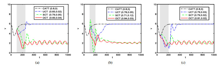
Figures(5)  /  Tables(4)

Other Articles By Authors

/

DownLoad:  Full-Size Img  PowerPoint
Return
Return

Catalog