
The present paper considers a fractional-order N species network, in which, the general functions are used for finding general theories. The existence, uniqueness, and non-negativity of the solutions for the considered model are proved. Moreover, the local and global asymptotic stability of the equilibrium point are studied by using eigenvalue method and Lyapunov direct method. Finally, some simple examples and numerical simulations are provided to demonstrate the theoretical results.
Citation: Yingkang Xie, Junwei Lu, Bo Meng, Zhen Wang. Stability analysis for a new fractional order N species network[J]. Mathematical Biosciences and Engineering, 2020, 17(4): 2805-2819. doi: 10.3934/mbe.2020154
[1] | B. Spagnolo, D. Valenti, A. Fiasconaro . Noise in ecosystems: A short review. Mathematical Biosciences and Engineering, 2004, 1(1): 185-211. doi: 10.3934/mbe.2004.1.185 |
[2] | Meng Fan, Bingbing Zhang, Michael Yi Li . Mechanisms for stable coexistence in an insect community. Mathematical Biosciences and Engineering, 2010, 7(3): 603-622. doi: 10.3934/mbe.2010.7.603 |
[3] | Yanjie Hong, Wanbiao Ma . Sufficient and necessary conditions for global attractivity and stability of a class of discrete Hopfield-type neural networks with time delays. Mathematical Biosciences and Engineering, 2019, 16(5): 4936-4946. doi: 10.3934/mbe.2019249 |
[4] | Yun Kang, Sourav Kumar Sasmal, Amiya Ranjan Bhowmick, Joydev Chattopadhyay . Dynamics of a predator-prey system with prey subject to Allee effects and disease. Mathematical Biosciences and Engineering, 2014, 11(4): 877-918. doi: 10.3934/mbe.2014.11.877 |
[5] | Yufei Wang, Huidong Cheng, Qingjian Li . Dynamic analysis of wild and sterile mosquito release model with Poincaré map. Mathematical Biosciences and Engineering, 2019, 16(6): 7688-7706. doi: 10.3934/mbe.2019385 |
[6] | N. H. AlShamrani, A. M. Elaiw . Stability of an adaptive immunity viral infection model with multi-stages of infected cells and two routes of infection. Mathematical Biosciences and Engineering, 2020, 17(1): 575-605. doi: 10.3934/mbe.2020030 |
[7] | Tainian Zhang, Zhixue Luo, Hao Zhang . Optimal harvesting for a periodic $ n $-dimensional food chain model with size structure in a polluted environment. Mathematical Biosciences and Engineering, 2022, 19(8): 7481-7503. doi: 10.3934/mbe.2022352 |
[8] | Balázs Boros, Stefan Müller, Georg Regensburger . Complex-balanced equilibria of generalized mass-action systems: necessary conditions for linear stability. Mathematical Biosciences and Engineering, 2020, 17(1): 442-459. doi: 10.3934/mbe.2020024 |
[9] | Salvatore Rionero . A nonlinear $L^2$-stability analysis for two-species population dynamics with dispersal. Mathematical Biosciences and Engineering, 2006, 3(1): 189-204. doi: 10.3934/mbe.2006.3.189 |
[10] | Shuixian Yan, Sanling Yuan . Critical value in a SIR network model with heterogeneous infectiousness and susceptibility. Mathematical Biosciences and Engineering, 2020, 17(5): 5802-5811. doi: 10.3934/mbe.2020310 |
The present paper considers a fractional-order N species network, in which, the general functions are used for finding general theories. The existence, uniqueness, and non-negativity of the solutions for the considered model are proved. Moreover, the local and global asymptotic stability of the equilibrium point are studied by using eigenvalue method and Lyapunov direct method. Finally, some simple examples and numerical simulations are provided to demonstrate the theoretical results.
Population dynamics is one of the main issues of theoretical biomathematics and has aroused the interest of many scholars in the fields of mathematical biology. A lot of methods have been presented and developed to study the evolution of population dynamics. It is clear that establishing mathematical models is the prerequisite for analysis of population dynamics. Until now, researchers have proposed a variety of models, represented by difference equations or differential equations [1,2,3].
As is well known, no species can exist in isolation, all populations must be related to the others directly or indirectly, and mutualism, parasitism, competition and predation are the four most widespread direct relationships in the ecosystem [4]. Based on these four relationships, researchers have established a variety of models to study the dynamics of the population, such as the Lotka-Volterra models, Leslie-Gower models and predator-prey models [5,6,7,8]. In recent years, many researchers began to study more complex and realistic population models and have got some interesting results [9,10,11,12,13,14]. In [15], a predator-prey system with Beddington-DeAngelis functional response was considered, and global asymptotical stability of the positive equilibrium was investigated by using divergency criterion. In [16], a ratio-dependent prey-predator model with the Allee effect was proposed, and bifurcation and stability analysis were carried out. Moreover, all possible non-degenerated phase portraits have been displayed. In [17], a simple predator-prey interaction where predator population is subjected to harvesting was considered, and different outcomes including switching of stability, oscillation and deterministic extinction were demonstrated.
On the other hand, with the development of fractional calculus, researchers have applied fractional derivatives to various fields [18,19,20,21,22,23,24,25,26,27,28,29]. Compared with the classical integer-order counterpart, fractional derivative is an outstanding instrument to describe memory and hereditary properties of various materials and processes [30]. In [31], the fractional-order predator-prey model and the fractional-order rabies model were firstly established. Moreover, existence and uniqueness of solutions, and stability of equilibrium points were studied. A comparison between the proposed fractional-order model and its integer-order counterpart was made. Since then, fractional population models have received extensive attention, and numerous results have been reported in the literature. Some different fractional Lotka-Volterra models are studied in [32,33,34]. For more details, see [35,36,37,38] and the references cited therein. In [39], stability of fractional-order nonlinear systems was studied by using Lyapunov direct method with the introduction of generalized Mittag-Leffler stability definition. It provided a new instrument to investigate the dynamics of the fractional population model. After that, the Lyapunov direct method has been widely applied to stability analysis of the fractional population model [40,41,42]. For instance, dynamics of a fractional-order predator-prey model incorporating a prey refuge was discussed in [40]. Stability of a fractional-order prey-predator system with time-delay and Monod-Haldane functional response was considered in [41]. Stability of a fractional-order two-species facultative mutualism model with harvesting was addressed in [42]. Some sufficient conditions to ensure the stability of the considered models were obtained in the aforementioned references based on the the Lyapunov direct method. Recent years, variety of interesting fractional-order population models are studied and some significant results were obtained [43,44,45].
Due to factors such as reproduction, most of the population systems have memory and hereditary effects. Thus, the fractional-order population system is more realistic than integer-order counterpart. Moreover, the integer-order system can be seemed as a special form of fractional-order system. So the analysis of fractional-order model is more general. Based on the above advantages, a new fractional-order N species model is established in this paper. In order to find general theories, the general functions are used in this model. It can be said that most of the population model can be seemed as a special form of this model. Therefore, it is valuable to analyze the stability of this model. The main contributions of this paper are as follows: First of all, a new generalized fractional order N species network is established to describe the relationship between species in an ecosystem. In addition, the existence, uniqueness and non-negativity of the solution are discussed. Moreover, the algebraic criteria for local stability and global stability are established by using the eigenvalue method and the Lyapunov direct method, respectively. Finally, the theoretical analysis is demonstrate by three examples and numerical simulations.
The rest of this paper is organized as follows. In Section 2, some definitions in fractional calculus and some stability results are introduced. In Section 3, existence, uniqueness, non-negativity of the solutions, and local and global asymptotical stability of the equilibrium point are discussed in depth. In Section 4, some numerical simulation results are presented. Finally, some conclusions are drawn in Section 5.
In this section, some definitions and lemmas in fractional calculus are recalled, which will be used later.
Definition 1. [46] The Caputo fractional derivative of a function f(t) with order α is defined as
Dαf(t)=1Γ(n−α)∫tt0f(n)(τ)(t−τ)α+1−ndτ, n−1<α<n, | (1) |
where α>0, t0 is the initial time, n∈N, and Γ is the Gamma function.
Lemma 1. [47] The equilibrium points x∗ of Dαx(t)=f(x) are locally asymptotically stable if all eigenvalues λi of the Jacobian matrix J=∂f/∂x evaluated at the equilibrium points satisfy |arg(λi)|>απ2.
Lemma 2. [48] Let x(t)∈R+ be a differentiable function. Then, for any time instant t≥t0
Dα[x(t)−x∗−x∗lnx(t)x∗]≤(1−x∗x(t))Dαx(t),x∗∈R+,∀α∈(0,1). | (2) |
Lemma 3. [49] (Uniform Asymptotic Stability Theorem) Let x=0 be an equilibrium point of Dαx(t)=f(t,x), and let Ω⊂Rn be a domain containing x=0. Let V(t,x):[t,∞)×Ω→R be a continuously differentiable function such that
W1(x)≤V(t,x)≤W2(x), | (3) |
and
DαV(t,x)≤−W3(x), | (4) |
for t≥0,x∈Ω and 0<α<1, where W1(x),W2(x) and W3(x) are continuous positive definite functions on Ω, then x=0 is uniformly asymptotically stable.
Remark 1. [39] If x=x∗ is the equilibrium point of Dαx(t)=f(t,x) and satisfies the conditions of Lemma 3, then x=x∗ is uniformly asymptotically stable.
In [50], the following model is considered.
u′i(t)=ui(t)[ai(t)−N∑j=1bij(t)uj(t)], i=1,2,…,N, | (5) |
where the functions ai(t),bij(t) are assumed to be nonnegative and continuous for t∈(−∞,∞). This system is commonly called the Volterra-Lotka system for N-competing species. Because of the complex relations between the species, it would be more realistic to change the functions bij(t)uj(t) to fij(uj(t)), so one can build a new population model.
This paper considers the following generalized fractional-order ecosystem model:
Dαxi(t)=Fi(x1,x2,…,xn)=xi(t)N∑j=1aijfij(xj(t)), | (6) |
xi(t0)=xit0,i=1,2,3,…,N, |
where t0≥0 is the initial time, xi(t) for i=1,2,3,…,N denotes population density of the species xi at time t, aij=±1,0. fij(xj(t)) are continuous, non-negative and differentiable functions.
fii(xi) are the specific growth rate of xi in the absence of other species for i=1,2,3,…,N. If xi represents a producer in ecosystems, one can see that the specific growth rate of xi is positive, so one makes aii>0(=1). If xi represents a consumer in ecosystems, one can see that the specific growth rate of xi is negative, so one makes aii<0(=−1). The greater the number of species is, the greater the intra-specific competition will be. So dfii(xi)/dxi<0, if xi represents a producer and dfii(xi)/dxi≥0, if xi represents a consumer.
fij(xj) are the effect of xj on xi in a time unit for i=1,2,3,…,N, i≠j. The greater xj is the greater the impact on xi will be, so one makes dfij(xj)/dxj>0. It is easy to see that when xj=0, there is no effect on xi. That is fij(xj)=0 for xj=0.
One can describe the relationship between xi and xj by determining the sign of aij and aji. If aij>0(=1) and aji>0(=1), then the relationship between xi and xj is mutualism. If aij>0(=1) and aji<0(=−1), then the relationship between xi and xj is predation(parasitism) and it can be seen that xi is the predator(parasite) and xj is the prey (host). If aij<0(=−1) and aji<0(=−1), then the relationship between xi and xj is competition. If aij=0 and aji=0, there is no direct relationship between xi and xj.
One should consider the significance of system (6), that is the boundedness of xi. So the function fij(xj(t)) for i,j=1,2,3,…,n should give the restriction of making xi to be bounded.
Remark 2. If xi represents a producer, since dfii(xi)/dxi<0 and fii(xi)>0, then fii(xi)=b+g(xi) (g(xi) does not contain a constant term and b is a constant), where b>0 represents growth and dg(xi)/dxi<0. In addition, if the time dependence of coefficients is ignored, Eq (5) can be regarded as a special form of Eq (6) (just set all xi as a producer, aii=1, aij=−1, fij(xj)=bijxj and α=1).
Remark 3. Moreover, let all xi as a producer, aii=1, aij=−1, fii=ki−kiciixi, fij=kicijxj for i,j=1,2,3 and i≠j, then Eq (6) is same as the model in [32]. Let x1 as a producer and x2 as a consumer, a11,a21=1, a12,a22=−1, f11=r−kx1, f12=x2, f21=βx1 and f22=1, then Eq (6) is same as system (5) in [33]. Let x1 as a producer and x2,x3 as consumers, ai1=1, aij=−1, f1j=c1jxj, fj1=cj1xj, , f11=b1−c11x1, fjj=bj+cjjxj for i=1,2,3,j=2,3, f23=c23x3 and f32=c32x2, then Eq (6) is same as system (1) in [34]. Just let a23=a32=0, then Eq (6) is same as system (19) in [34]. So the models in [32,33,34] are special forms of Eq (6).
Theorem 1. If xi(t0)>0, for i=1,⋯,N, then is a unique solution x(t) of system (6) in RN+ for t≥t0.
Proof. We study the existence and uniqueness of the solution of system (6) in the region Ω×[0,T], where Ω={(x1,x2,…,xN)∈R3:max{∣x1∣,∣x2∣,…,∣xN∣<M}} and T<+∞. Denote X=(x1(t1),x2(t1),…,xN(t1)) and ˉX=(x1(t2),x2(t2),…,xN(t2)). Consider a mapping H(X)=(H1(X),H2(X),…,HN(X)) where
Hi(X)=xi(t)N∑j=1aijfij(xj(t)) |
For any X,ˉX∈Ω
‖H(X)−H(ˉX)‖=N∑i=1|xi(t1)N∑j=1aijfij(xj(t1))−xi(t2)N∑j=1aijfij(xj(t2))|=N∑i=1|xi[N∑j=1aijfij(xj(t1))−N∑j=1aijfij(xj(t2))]+[xi(t1)−xi(t2)]N∑j=1aijfij(xj(t2))|≤N∑i=1|M[N∑j=1aijfij(xj(t1))−N∑j=1aijfij(xj(t2))]+[xi(t1)−xi(t2)]N∑j=1aijfij(xj(t2))|≤N∑i=1|MN∑j=1aijfij(xj(t))[xj(t1)−(xj(t2))]+[xi(t1)−xi(t2)]N∑j=1aijfij(xj(t2))|≤|MN∑i=1N∑j=1aijfij(xj(t))[xj(t1)−(xj(t2))]+N∑i=1N∑j=1[xi(t1)−xi(t2)]aijfij(xj(t2))|≤N∑i=1N∑j=1|Mfji(xi(t))[xi(t1)−(xi(t2))]|+N∑i=1N∑j=1|[xi(t1)−xi(t2)]fij(xj(t2))|≤L‖X−ˉX‖ |
where t∈[t1,t2] and L=max{M∑Nj=1[fji(xi(t))−fij(xj(t2))]} for i=1,2,…,n. Obviously, H(Z) satisfies the Lipschitz condition. Thus, system (6) has a unique solution x(t).
Theorem 2. If xi(t0)>0, for i=1,⋯,N, then solutions of system (6) are non-negative.
Proof. Let xi(t0)>0,i=1,⋯,N in RN+ be the initial solution of system (6). By contradiction, suppose that there exists a solution x(t) that lies outside of RN+. The consequence is that x(t) crosses the xi axis for i=1,2,3,…,N.
Assume that x(t) crosses xk=0, then there exists t∗ such that t∗>t0 and xk(t∗)=0, and there exists t1 sufficiently close to t∗ such that t1>t∗, and xk(t)<0 for all t∈(t∗,t1]. Based on the k-th equation of system (6), one obtains
Dαxk(t)=xk(t)N∑j=1akjfkj(xj(t)). | (8) |
Since x(t) and fkj(xj(t)) are continuous, one can see that fkj(xj(t)) is bounded on t∈[t∗,t1].
Assume that max|akjfkj(xj(t))|=M. Then
Dαxk(t)≥xk(t)(nM). | (9) |
By using the Laplace transform on both sides, one gets
xk(t)≥xk(t∗)Eα(nM(t−t∗)α),t∈[t∗,t1], | (10) |
where Eα is the Mittag-Leffler function. Thus, x(t)≥0 for any t≥t0, which contradicts the assumption. By using the same method, one gets xi(t) are non-negative for i=1,2,…,N.
In this section, the stability of the equilibrium points will be investigated by using the Lyapunov direct method. The equilibrium points of the model can be obtained from the following equations.
xi(t)N∑j=1aijfij(xj(t))=0i=1,2,3,…,N. | (11) |
In the following, we will only consider the stability of a certain equilibrium point, for the other equilibrium points can be discussed by the same way.
Assume that x∗ is the equilibrium point of system (6), then it has k (0≤k≤N) components of vector x∗ that are not 0. By the operations of row and column, x∗ can be written as x∗=(x∗1,x∗2,…,x∗k,0,…,0). The Jacobian matrix at x∗ is
J(x∗)=[b11b12b13⋯ b1kb1k+1b1k+2⋯b1nb21b22b23⋯ b2kb2k+1b2k+2⋯b2nb31b32b33⋯ b3kb3k+1b3k+2⋯b3n⋮⋮⋮⋱⋮⋮⋮⋱⋮bk1bk2bk3⋯ bkkbkk+1bkk+2⋯bkn000⋯ 0∑nj=1ak+1′jfk+1′j(x∗j)0⋯0000⋯ 00∑nj=1ak+2′jf(k+2′j)(x∗j)⋯0⋮⋮⋮⋱⋮⋮⋮⋱⋮000⋯ 000⋯∑nj=1anjfnj(x∗j)], | (12) |
where bij=aijf′ij(x∗j)x∗i.
Solving the characteristic equation det(λI−J(x∗))=0 for λ to find the eigenvalues of J(x∗), one gets
[λk+a1λk−1+a2λk−2+⋯+ak−1λ+ak][(λ−n∑j=1ak+1′jfk+1′j(x∗j))⋯(λ−n∑j=1anjfnj(x∗j))]=0. | (13) |
Let
A=[b11b12b13⋯ b1kb21b22b23⋯ b2kb31b32b33⋯ b3k⋮⋮⋮⋱⋮bk1bk2bk3⋯ bkk], | (14) |
M(i,j) is the j−th i−order principal minor of A and ai=(−1)i∑Cikj=1M(i,j).
For the sake of discussion, we define Hj as follows
Hj=|a1a3a5⋯ a2j−11a2a4⋯ a2j−20a1a3⋯ a2j−301a2⋯ a2j−4⋮⋮⋮⋱⋮000⋯ aj|, | (15) |
Theorem 3. Suppose that x∗=(x∗1,x∗2,…,x∗k,0,…,0) is the equilibrium point of the system (6), then the equilibrium point is locally asymptotically stable, if the following algebraic conditions hold:
1). ∑kj=1aijfij(x∗j)+aiifii(x∗j)≤0, for i=k+1,k+2,…,N.
2). ai for i=1,2,…,k satisfy Hj>0 for j=1,2,…,k.
Proof. According to the Hurwitz criterion, if Hj>0 for j=1,2,…,k, then all eigenvalues of λk+a1λk−1+a2λk−2+⋯+ak−1λ+ak=0 have negative real part.
According to ∑kj=1aijfij(x∗j)+aiifii(x∗j)≤0, one can see that all eigenvalues of [(λ−∑nj=1ak+1′jfk+1′j(x∗j))⋯(λ−∑nj=1anjfnj(x∗j))]=0 are negative or equal to 0.
Above all, the equilibrium point is locally asymptotically stable.
Remark 4. The conditions of Theorem 3 are sufficient conditions. If Hj<0 and all eigenvalues of λk+a1λk−1+a2λk−2+⋯+ak−1λ+ak=0 satisfy the condition in Lemma 1, the equilibrium point is also locally asymptotically stable.
Theorem 4. Suppose that x∗=(x∗1,x∗2,…,x∗k,0,…,0) is the equilibrium point of system (6), then x∗ is globally asymptotically stable, if the following algebraic conditions hold:
1). x∗ satisfy ∑kj=1aijfij(x∗j)+aiifii(x∗j)≤0, for i=k+1,k+2,…,N.
2). ∃kij≥0 satisfy ∑nj=1kij=1 for i,j=1,2,…,N and i≠j.
3). ∃ci>0 and ∃kij≥0 satisfy 2√aiiajjcicjkijkjif′ii(x∗i)f′jj(x∗j)>|aijcif′ij(x∗j)+ajicjf′ji(x∗i)| for i,j=1,2,…,N.
Proof. If ∑kj=1aijfij(x∗j)+aiifii(x∗j)≤0, for i=k+1,k+2,…,N, that is
{n∑j=1aijfij(x∗j)=0,fori=1,2,…,k,n∑j=1aijfij(x∗j)≤0,fori=k+1,k+2,…,N. |
Let us consider the following positive definite function about x∗
V(x1,x2,…,xn)=k∑i=1ci(xi−x∗i−x∗ilnxix∗i)+n∑i=k+1cixi. | (16) |
One can subtly choose ci>0 such that V is a Lyapunov function. By Lemma 2, one obtains
DαV(x1,x2,…,xn)≤k∑i=1n∑j=1ci(xi−x∗i)(aijfij(xj(t)))+n∑i=k+1n∑j=1cixi(aijfij(xj(t)))≤k∑i=1n∑j=1ci(xi−x∗i)(aijfij(xj)−aijfij(x∗j))+n∑i=k+1n∑j=1ci(xi−x∗i)(aijfij(xj)−aijfij(x∗j)). | (17) |
For arbitrary ε>0, since functions fij for i,j=1,2,…,n are differentiable functions, there exists δ>0 such that |xi−x∗i|<δ for i=1,2,…,N, it implies
|fij(xj)−fij(x∗j)xj−x∗j−f′ij(x∗j)|<εfori,j=1,2,…,n. | (18) |
Thus
DαV(x1,x2,…,xn)≤n∑i=1n∑j=1ci(xi−x∗i)(xj−x∗j)(aijf′ij(x∗j)+ε) | (19) |
By the arbitrariness of ε, one has
DαV(x1,x2,…,xn)≤n∑i=1n∑j=1ci(xi−x∗i)(xj−x∗j)aijf′ij(x∗j)=n∑i=1n∑j=1[(kijaiici(xi−x∗i)2f′ii(x∗i)+(xi−x∗i)(xj−x∗j)(ciaijf′ij(x∗j)+cjajif′ji(x∗i))2]. | (20) |
For i≠j, then one has
DαV(x1,x2,…,xn)≤−n∑i=1n∑j>i[2|xi−x∗i||xj−x∗j|√aiiajjcicjkijkjif′ii(x∗i)f′jj(x∗j)−(xi−x∗i)(xj−x∗j)(ciaijf′ij(x∗j)+cjajif′ji(x∗i))]. | (21) |
According to the condition 2√aiiajjcicjkijkjif′ii(x∗i)f′jj(x∗j)>|aijcif′ij(x∗j)+ajicjf′ji(x∗i)|, and aiif′ii(xi)<0 for i=1,2,…,n. So the conditions in Lemma 3 are satisfied, where W3(x)=∑ni=1∑nj>i[2|xi−x∗i||xj−x∗j|√aiiajjcicjkijkjif′ii(x∗i)f′jj(x∗j)−(xi−x∗i)(xj−x∗j)(ciaijf′ij(x∗j)+cjajif′ji(x∗i))]>0.
Thus, x∗ is a globally asymptotically stable equilibrium point for the system (6).
Remark 5. According to theorem 4, one can see that N-order system should have N(N−1)/2 conditions at least. So if N is large enough, it is difficult to find the suitable ci,kij for i,j=1,2,3,…,n and i≠j.
In this section, we will give some examples to demonstrate the theoretical analysis.
Example 1:
Let us consider the functions of the system (6) as follow
f11(x1(t))=2(2−x1(t)),f12(x2(t))=x2(t),f13(x3(t))=x3(t),a11=1,a12=−1,a13=−1,f21(x1(t))=x1(t),f22(x2(t))=2(2−x2(t)),f23(x3(t))=x3(t),a21=−1,a22=1,a23=−1,f31(x1(t))=x1(t),f32(x2(t))=x2(t),f33(x3(t))=2(2−x3(t)),a31=−1,a32=−1,a33=1. | (22) |
Therefore, the system (6) can be denoted by the following Volterra-Lotka competition system:
Dαx1(t)=x1(t)(4−2x1(t)−x2(t)−x3(t)),Dαx2(t)=x2(t)(4−x1(t)−2x2(t)−x3(t)),Dαx3(t)=x3(t)(4−x1(t)−x2(t)−2x3(t)). | (23) |
From the parameters of the system, it can be seen that the equilibrium points of the system are (1,1,1), (1,1,0) and (1,0,0). One can see that when kij=0.5 and ci=1 for i,j=1,2,3,i≠j, the equilibrium point x∗=(1,1,1) can satisfy three conditions in Theorem 4. Other equilibrium points can not satisfy condition 1 in Theorem 4. One selects the initial values as (0.8,0.6,0.4), (1.6,1.2,0.8), (2.4,1.8,1.2) and (3.2,2.4,1.6) respectively, and the numerical results are shown in Figure 1. From Figure 1, one can see that the positive equilibrium point (1, 1, 1) of system (23) is globally asymptotically stable.
Example 2:
In this example, one considers the functions fij of system (6) as nonlinear form:
f11(x1(t))=2(2−x21(t)),f12(x2(t))=x22(t),f13(x3(t))=x23(t),a11=1,a12=−1,a13=−1,f21(x1(t))=x21(t),f22(x2(t))=2(2−x22(t)),f23(x3(t))=x23(t),a21=−1,a22=1,a23=−1,f31(x1(t))=x21(t),f32(x2(t))=x22(t),f33(x3(t))=2(2−x23(t)),a31=−1,a32=−1,a33=1. | (24) |
Therefore, the system (6) can be denoted by the following competition system:
Dαx1(t)=x1(t)(4−2x21(t)−x22(t)−x23(t)),Dαx2(t)=x2(t)(4−x21(t)−2x22(t)−x23(t)),Dαx3(t)=x3(t)(4−x21(t)−x22(t)−2x23(t)). | (25) |
From the parameters of the system, it can be seen that the equilibrium points of the system are (1,1,1) and (0,0,0). One can see that when kij=0.5 and ci=2 for i,j=1,2,3,i≠j, the equilibrium point x∗=(1,1,1) can satisfy three conditions in Theorem 4 and the other can not satisfy all conditions in Theorem 4. One selects the initial values as (0.4,0.6,0.5), (0.8,1.2,1), (1.2,1.8,1.5) and (1.6,2.4,2) respectively, and the numerical results are shown in Figure 2. From Figure 2, one can see that the positive equilibrium point (1, 1, 1) of system (25) is globally asymptotically stable.
Example 3:
The new example will consider the complex relationships between the species, one selects the functions of the system (6) as follow.
f11(x1(t))=0.5(1−x1(t)),f12(x2(t))=x2(t),f13(x3(t))=x3(t),a11=1,a12=−1,a13=−1,f21(x1(t))=x1(t),f22(x2(t))=x2(t),f23(x3(t))=x3(t),a21=1,a22=−1,a23=−1,f31(x1(t))=x1(t),f32(x2(t))=0.5x2(t),f33(x3(t))=2x3(t).a31=1,a32=−1,a33=−1. |
Therefore, the system (6) can be denoted by the following prey-predator system with interspecific competition:
Dαx1(t)=x1(t)(0.5(1−x1(t))−x2(t)−x3(t)),Dαx2(t)=x2(t)(x1(t)−x2(t)−x3(t)),Dαx3(t)=x3(t)(x1(t)−0.5x2(t)−2x3(t)). | (26) |
From the parameters of the system, it can be seen that the equilibrium points of the system are (1/3,2/9,1/9), (1/3,1/3,0) and (1,0,0). One can see that when k12=k21=0.5, k32=k23=0.8, k21=k31=0.2 and ci=1 for i,j=1,2,3,i≠j, the equilibrium point (1/3,2/9,1/9) can satisfy three conditions in Theorem 4. One takes initial values (0.2,0.2,0.3), (0.4,0.4,0.6), (0.6,0.6,0.9) and (0.8,0.8,1.2) respectively, and the numerical results are shown in Figure 3. From Figure 3, one can see that the positive equilibrium point (1/3,2/9,1/9) of system (26) is globally asymptotically stable.
In this paper, one considers a class of generalized fractional population model. Firstly, the existence, uniqueness and non-negative of solutions of the system are proved. Secondly, one provides a sufficient conditions for local stability and globally stability of the equilibrium points. Finally, three examples are given to demonstrate the theoretical analysis. This paper not only extends the integer population models to fractional-order form, but also extends the dimension to n-dimension. The new model can be used to simulate the relationships between various populations in a complex ecosystem. Compared with other population models, our model is more general.
Time delay stays in the biological system widely and may effect the stability of the biological system. Thus, system (6) with time delay is of great research value. It will be our future work.
This work was supported by the National Natural Science Foundation of China (Nos. 61573008, 61973199), the Natural Science Foundation of Shandong Province (No. ZR2018MF005), and the SDUST graduate innovation project (No. SDKDYC190353).
The author declares no conflicts of interest in this paper.
[1] | F. Peter, Modelling with differential and difference equations, Cambridge University Press, Cambridge, 1997. |
[2] |
T. Zhang, T. Zhang, X. Meng, Stability analysis of a chemostat model with maintenance energy, Appl. Math. Lett., 68 (2017), 1-7. doi: 10.1016/j.aml.2016.12.007
![]() |
[3] |
X. Wang, Z. Wang, H. Shen, Dynamical analysis of a discrete-time SIS epidemic model on complex networks, Appl. Math. Lett., 94 (2019), 292-299. doi: 10.1016/j.aml.2019.03.011
![]() |
[4] | X. Zhao, Dynamical systems in population biology, Springer, New York, 2000. |
[5] |
T. Zhang, X. Liu, X. Meng, T. Zhang, Spatio-temporal dynamics near the steady state of a planktonic system, Comput. Math. Appl., 75 (2018), 4490-4504. doi: 10.1016/j.camwa.2018.03.044
![]() |
[6] | X. Yu, S. Yuan, T. Zhang, Survival and ergodicity of a stochastic phytoplankton-zooplankton model with toxin producing phytoplankton in an impulsive polluted environment, Appl. Math. Comput., 347 (2019), 249-264. |
[7] |
T. Zhang, Y. Xing, H. Zang, M. Han, Spatio-temporal patterns in a predator-prey model with hyperbolic mortality, Nonlinear Dyn., 78 (2014), 265-277. doi: 10.1007/s11071-014-1438-6
![]() |
[8] |
C. L. Wolin, L. R. Lawlor, Models of facultative mutualism: density effects, Am. Nat., 124 (1984), 843-862. doi: 10.1086/284320
![]() |
[9] |
S. Ahmad, A. C. Lazer, Average growth and total permanence in a competitive Lotka-Volterra System, Ann. Mat. Pura. Appl., 185 (2006), S47-S67. doi: 10.1007/s10231-004-0136-2
![]() |
[10] |
T. K. Kar, H. Matsuda, Global dynamics and controllability of a harvested prey-predator system with Holling type Ⅲ functional response, Nonlinear Anal.-Hybrid Syst., 1 (2007), 59-67. doi: 10.1016/j.nahs.2006.03.002
![]() |
[11] | I. Al-Darabsah, X. Tang, Y. Yuan, A prey-predator model with migrations and delays, Discrete Contin. Dyn. Syst.-Ser. B, 21 (2017), 737-761. |
[12] |
B. I. Camara, M. Haque, H. Mokrani, Patterns formations in a diffusive ratio-dependent predatorprey model of interacting populations, Physica A, 461 (2016), 374-383. doi: 10.1016/j.physa.2016.05.054
![]() |
[13] |
G. M. Abernethy, R. Mullan, D. H. Glass, M. Mccartney, A multiple phenotype predator-prey model with mutation, Physica A, 465 (2017), 762-774. doi: 10.1016/j.physa.2016.08.037
![]() |
[14] |
P. S. Mandal, Noise-induced extinction for a ratio-dependent predator-prey model with strong Allee effect in prey, Physica A, 496 (2018), 40-52. doi: 10.1016/j.physa.2017.12.057
![]() |
[15] |
T. W. Hwang, Global analysis of the predator-prey system with Beddington-DeAngelis functional response, J. Math. Anal. Appl., 281 (2003), 395-401. doi: 10.1016/S0022-247X(02)00395-5
![]() |
[16] |
M. Sen, M. Banerjeea, A. Morozov, Bifurcation analysis of a ratio-dependent prey-predator model with the Allee effect, Ecol. Complex, 11 (2012), 12-27. doi: 10.1016/j.ecocom.2012.01.002
![]() |
[17] |
S. Chakraborty, S. Pal, N. Bairagi, Predator-prey interaction with harvesting: mathematical study with biological ramifications, Appl. Math. Model., 36 (2012), 4044-4059. doi: 10.1016/j.apm.2011.11.029
![]() |
[18] |
X. Huang, Y. Fan, J. Jia, Z. Wang, Y. Li, Quasi-synchronization of fractional-order memristorbased neural networks with parameter mismatches, IET Contr. Theory Appl., 11 (2017), 2317-2327. doi: 10.1049/iet-cta.2017.0196
![]() |
[19] |
J. Jia, X. Huang, Y. Li, J. Cao, A. Alsaedi, Global Stabilization of Fractional-Order MemristorBased Neural Networks with Time Delay, IEEE Trans. Neural Netw. Learn. Syst., 31 (2020), 997-1009. doi: 10.1109/TNNLS.2019.2915353
![]() |
[20] | Y. Fan, X. Huang, Z. Wang, Nonlinear dynamics and chaos in a simplified memristor-based fractional-order neural network with discontinuous memductance function, Nonlinear Dyn., 9 (2018), 1-17. |
[21] |
C. Huang, L. Cai, J. Cao, Linear control for synchronization of a fractional-order time-delayed chaotic financial system, Chaos Soliton. Fract., 113 (2018), 326-332. doi: 10.1016/j.chaos.2018.05.022
![]() |
[22] |
X. Wang, Z. Wang, J. Xia, Stability and bifurcation control of a delayed fractional-order ecoepidemiological model with incommensurate orders, J. Frankl. Inst.-Eng. Appl. Math., 356 (2019), 8278-8295. doi: 10.1016/j.jfranklin.2019.07.028
![]() |
[23] |
A. Alkhazzan, P. Jiang, D. Baleanu, H. Khan, A. Khan, Stability and existence results for a class of nonlinear fractional differential equations with singularity, Math. Meth. Appl. Sci., 41 (2018), 9321-9334. doi: 10.1002/mma.5263
![]() |
[24] |
X. Wang, Z. Wang, X. Huang, Y. Li, Dynamic analysis of a delayed fractional-order SIR model with saturated incidence and treatment functions, Int. J. Bifurcat. Chaos, 28 (2018), 1850180. doi: 10.1142/S0218127418501808
![]() |
[25] | A. Yusuf, A. I. Aliyu, D. Baleanu, Conservation laws, soliton-like and stability analysis for the time fractional dispersive long-wave equation, Adv. Differ. Equ., 1 (2018), 319. |
[26] |
Y. Xie, J. Lu, Z. Wang, Stability analysis of a fractional-order diffused prey-predator model with prey refuges, Physica A, 526 (2019), 120773. doi: 10.1016/j.physa.2019.04.009
![]() |
[27] | Z. Wang, Y. Xie, J. Lu, Y. Li, Stability and bifurcation of a delayed generalized fractional-order prey-predator model with interspecific competition, Appl. Math. Comput., 347 (2019), 360-369. |
[28] |
G. C. Wu, D. Baleanu, L. L. Huang, Novel Mittag-Leffler stability of linear fractional delay difference equations with impulse, Appl. Math. Lett., 82 (2018), 71-78. doi: 10.1016/j.aml.2018.02.004
![]() |
[29] |
C. N. Angstmann, A. M. Erickson, B. I. Henry, A. V. McGann, J. M. Murray, J. A. Nichols, Fractional order compartment models, SIAM J. Appl. Math., 77 (2017), 430-446. doi: 10.1137/16M1069249
![]() |
[30] | E. Ahmed, A. S. Elgazzar, On fractional order differential equations model for nonlocal epidemics, Physica A, 379 (2012), 607-614. |
[31] |
E. Ahmed, A. M. A. El-Sayed, H. A. A. El-Saka, Equilibrium points, stability and numerical solutions of fractional-order predator-prey and rabies models, J. Math. Anal. Appl., 325 (2007), 542-553. doi: 10.1016/j.jmaa.2006.01.087
![]() |
[32] | C. Guo, S. Fang, Stability and approximate analytic solutions of the fractional Lotka-Volterra equations for three competitors, Adv. Differ. Equ., 1 (2016), 219. |
[33] |
A. A. Elsadany, A. E. Matouk, Dynamical behaviors of fractional-order Lotka-Volterra predatorprey model and its discretization, J. Appl. Math. Comput., 49 (2015), 269-283. doi: 10.1007/s12190-014-0838-6
![]() |
[34] | J. Tian, Y. Yu, H. Wang, Stability and bifurcation of two Kinds of three-dimensional fractional Lotka-Volterra systems, Math. Probl. Eng., 2014 (2014). |
[35] | H. L. Li, L. Zhang, C. Hu, Y. L. Jiang, Z. Teng, Dynamical analysis of a fractional-order predatorprey model incorporating a prey refuge, J. Math. Anal. Appl., 54 (2016), 1-15. |
[36] |
D. Hu, H. Cao, Stability and bifurcation analysis in a predator-prey system with Michaelis-Menten type predator harvesting, Nonlinear Anal.-Real. World Appl., 33 (2017), 58-82. doi: 10.1016/j.nonrwa.2016.05.010
![]() |
[37] |
C. Huang, Z. Li, D. Ding, J. Cao, Bifurcation analysis in a delayed fractional neural network involving self-connection, Neurocomputing, 314 (2018), 186-197. doi: 10.1016/j.neucom.2018.06.016
![]() |
[38] |
C. Huang, X. Song, B. Fang, M. Xiao, J. Cao, Modeling, analysis and bifurcation control of a delayed fractional-order predator-prey model, Int. J. Bifurcat. Chaos, 28 (2018), 1850117. doi: 10.1142/S0218127418501171
![]() |
[39] |
Y. Li, Y. Q. Chen, I. Podlubny, Stability of fractional-order nonlinear dynamic systems: Lyapunov direct method and generalized Mittag-Leffler stability, Comput. Math. Appl., 59 (2010), 1810-1821. doi: 10.1016/j.camwa.2009.08.019
![]() |
[40] | G. P. Samanta, A. Maiti, M. Das, Stability analysis of a prey-predator fractional order model incorporating prey refuge, Ecol. Genet. Genomics, 7 (2018), 33-46. |
[41] |
R. Chinnathambi, F. A. Rihan, Stability of fractional-order prey-predator system with time-delay and Monod-Haldane functional response, Nonlinear Dyn., 92 (2018), 1-12. doi: 10.1007/s11071-018-4140-2
![]() |
[42] | N. Supajaidee, S. Moonchai, Stability analysis of a fractional-order two-species facultative mutualism model with harvesting, Adv. Differ. Equ., 1 (2017), 372. |
[43] |
J. Alidousti, Stability and bifurcation analysis for a fractional prey-predator scavenger model, Appl. Math. Model., 81 (2020), 342-355. doi: 10.1016/j.apm.2019.11.025
![]() |
[44] |
C. Huang, H. Li, T. Li, S. Chen, Stability and bifurcation control in a fractional predator-prey model via extended delay feedback, Int. J. Bifurcat. Chaos, 29 (2019), 1950150. doi: 10.1142/S0218127419501505
![]() |
[45] | X. Wang, Z. Wang, X. Shen, Stability and Hopf bifurcation of a fractional-order food chain model with disease and two delays, J. Comput. Nonlinear Dyn., 15 (2020). |
[46] | I. Podlubny, Fractional differential equations, Academic press, New York, 1999. |
[47] |
G. Ji, Q. Ge, J. Xu, Dynamic behaviors of a fractional order two-species cooperative systems with harvesting, Chaos Soliton. Fract., 92 (2016), 51-55. doi: 10.1016/j.chaos.2016.09.014
![]() |
[48] |
C. Vargas-De-Len, Volterra-type Lyapunov functions for fractional-order epidemic systems, Commun. Nonlinear Sci. Numer. Simul., 24 (2015), 75-85. doi: 10.1016/j.cnsns.2014.12.013
![]() |
[49] | H. Delavari, D. Baleanu, J. Sadati, Stability analysis of Caputo fractional-order nonlinear systems revisited, Nonlinear Dyn., 67 (2011), 2433-2439. |
[50] | S. Ahmad, A. C. Lazer, On the nonautonomous N-competing species problems, Appl. Anal., 57 (2007), 309-323. |
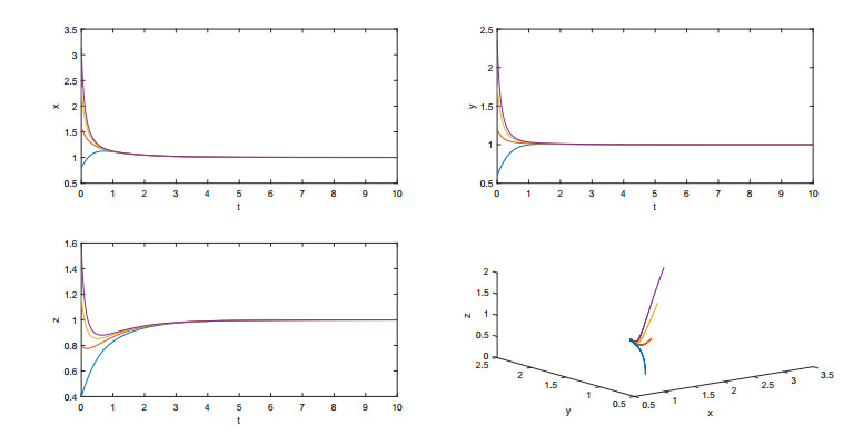
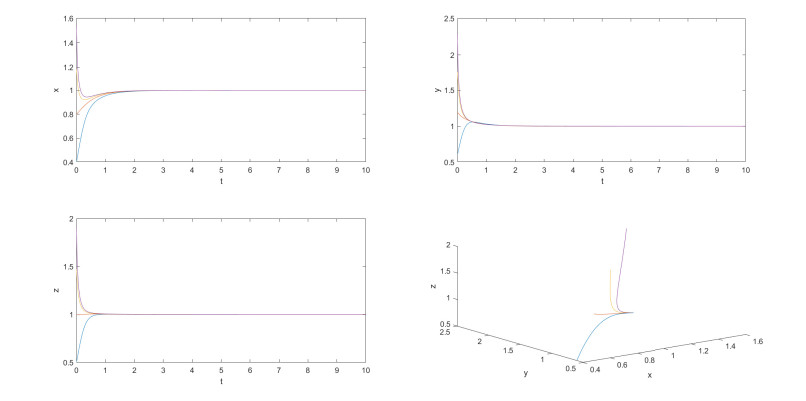
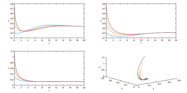
1. | Yingkang Xie, Zhen Wang, Junwei Lu, Yuxia Li, Stability analysis and control strategies for a new SIS epidemic model in heterogeneous networks, 2020, 383, 00963003, 125381, 10.1016/j.amc.2020.125381 |