Citation: József Z. Farkas, Gary T. Smith, Glenn F. Webb. A dynamic model of CT scans for quantifying doubling time of ground glass opacities using histogram analysis[J]. Mathematical Biosciences and Engineering, 2018, 15(5): 1203-1224. doi: 10.3934/mbe.2018055
[1] | Catherine S. Jarnevich, Tracy R. Holcombe, Catherine Cullinane Thomas, Leonardo Frid, Aaryn Olsson . Simulating long-term effectiveness and efficiency of management scenarios for an invasive grass. AIMS Environmental Science, 2015, 2(2): 427-447. doi: 10.3934/environsci.2015.2.427 |
[2] | Sonia Prestamburgo, Filippo Sgroi, Adriano Venudo, Carlo Zanin . Universal design as resilient urban space plan strategy. New scenarios for environmental resources' sustainable management. AIMS Environmental Science, 2021, 8(4): 321-340. doi: 10.3934/environsci.2021021 |
[3] | Laura Romero, Modesto Pérez-Sánchez, P. Amparo López-Jiménez . Improvement of sustainability indicators when traditional water management changes: a case study in Alicante (Spain). AIMS Environmental Science, 2017, 4(3): 502-522. doi: 10.3934/environsci.2017.3.502 |
[4] | Amir Hedayati Aghmashhadi, Giuseppe T. Cirella, Samaneh Zahedi, Azadeh Kazemi . Water resource policy support system of the Caspian Basin. AIMS Environmental Science, 2019, 6(4): 242-261. doi: 10.3934/environsci.2019.4.242 |
[5] | Miguel Mora-Pérez, Ignacio Guillen-Guillamón, Petra Amparo López-Jiménez . A CFD study for evaluating the effects of natural ventilation on indoor comfort conditions. AIMS Environmental Science, 2017, 4(2): 289-309. doi: 10.3934/environsci.2017.2.289 |
[6] | Beatriz Gullón, Belén Gómez, José Luis Alonso, Remedios Yáñez . Environmentally friendly technologies for obtaining high sugars concentrations from invasive woody species. AIMS Environmental Science, 2015, 2(4): 884-898. doi: 10.3934/environsci.2015.4.884 |
[7] | Novi Sylvia, Husni Husin, Abrar Muslim, Yunardi, Aden Syahrullah, Hary Purnomo, Rozanna Dewi, Yazid Bindar . Design and performance of a cyclone separator integrated with a bottom ash bed for the removal of fine particulate matter in a palm oil mill: A simulation study. AIMS Environmental Science, 2023, 10(3): 341-355. doi: 10.3934/environsci.2023020 |
[8] | Winai Meesang, Erawan Baothong, Aphichat Srichat, Sawai Mattapha, Wiwat Kaensa, Pathomsorn Juthakanok, Wipaporn Kitisriworaphan, Kanda Saosoong . Effectiveness of the genus Riccia (Marchantiophyta: Ricciaceae) as a biofilter for particulate matter adsorption from air pollution. AIMS Environmental Science, 2023, 10(1): 157-177. doi: 10.3934/environsci.2023009 |
[9] | Martina Grifoni, Francesca Pedron, Gianniantonio Petruzzelli, Irene Rosellini, Meri Barbafieri, Elisabetta Franchi, Roberto Bagatin . Assessment of repeated harvests on mercury and arsenic phytoextraction in a multi-contaminated industrial soil. AIMS Environmental Science, 2017, 4(2): 187-205. doi: 10.3934/environsci.2017.2.187 |
[10] | Afshin Meraj, Tina Shoa, Fereshteh Sadeghi Naieni Fard, Hassan Mina . A comprehensive bi-objective optimization model to design circular supply chain networks for sustainable electric vehicle batteries. AIMS Environmental Science, 2024, 11(2): 279-303. doi: 10.3934/environsci.2024013 |
It is now widely believed that the actual spread of many infectious diseases occurs in a diverse or dispersed population [1]. Subpopulations (or compartments) can be determined not only on the basis of disease-related factors such as mode of transmission, latent period, infectious period, and genetic susceptibility or resistance, but also on the basis of social, cultural, economic, demographic, and geographic factors [2]. In the viewpoint of epidemiology above, let S(t), I(t) and R(t) be the density of susceptible, infectious and recover individuals at time t, respectively, and we suppose that the dynamics of the disease transmission is governed by the following equations:
{dSdt=μN−g(S,I)−μS+γR,dIdt=g(S,I)−(μ+δ)I,dRdt=δI−μR−γR, | (1.1) |
where μ,δ,γ are all positive constants, μ the birth and death rate, δ the recovery rate of infectious individuals, and γ the rate of removed individuals who lose immunity and return to susceptible individuals class. Here, we assume that the disease does not have vertical transmission and is generally non–pathogenic and ignores the death induced by the disease. The infectious individuals force g(S,I) plays a key role in determining disease dynamics [3,4]. Traditionally, the density-dependent transmission (or the bilinear incidence rate, g(S,I)=βSI, and β is the proportionality constant) and the frequency-dependent transmission (or the standard incidence rate, g(S,I)=βSIS+I) are two extreme forms of disease transmission, which have been frequently used in well-known epidemic models [5,6,7]. There are several different nonlinear transmission functions proposed by researchers, to see more details, we refer to [8,9,10,11,12] and the references therein. Especially, Yuan and Li [13] studied a ratio-dependent nonlinear incident rate which takes the following form (1.2):
g(S,I)=f(IS)S=β(I/S)l1+α(I/S)hS=βSh−l+1IlSh+αIh, | (1.2) |
where the parameters l and h are positive constant, α is the parameter which measures the psychological or inhibitory effect. It is worthy to note that in the special case of α=1 and h=l=1, (1.2) becomes the well–known frequency-dependent transmission rate βSIS+I. In this case, the nonlinear incidence rate (1.2) can be seen as an extension form of the frequency-dependent transmission rate.
Before 1970s, ecological population modelers (involving epidemic models) typically used ordinary differential equations (ODE, e.g. model (1.1)), seeking equilibria and analyzing stability. These models provided important insights, such as when species can stably coexist and when susceptible and infectious densities oscillate over time [14]. The ODE models that have been described so far assume that the populations experience the same homogeneous environment. In reality, individual organisms are distributed in space and typically interact with the physical environment and other organisms in their spatial neighborhood [15]. More recently, many studies have shown that the spatial epidemic model is an appropriate tool for investigating the fundamental mechanism of complex spatiotemporal epidemic dynamics. In these studies, reaction-diffusion equations have been intensively used to describe spatiotemporal dynamics [16,17,18,19,20,21,22,23,24,25].
Many studies show that spatial heterogeneity generated by species dynamics is mathematically more interesting and also biologically more important [14]. In fact, relationships between individual-level processes and ecological dynamics often depend on population spatial structure, and epidemic dynamics can be governed by localized spatial processes of contact between susceptible and infectious individuals [27]. It has been suggested that spatial heterogeneity may address many of the deficiencies of epidemic models and play an important role in the spread of an epidemic [16,28,29,30,31,32,34,33]. Of them, Grenfell, Bjornstad and Kappey [31] showed that measles waves spreading from large cities to small towns in England and Wales are determined by the spatial hierarchy of the host population structure; Keeling et al. [32] showed that the spatial distribution of farms influences the regional variability of foot-and-mouth outbreaks in UK; Hufnagel et al. [34], Colizza et al. [33] showed that the high degree of predictability of the worldwide spread of infectious diseases is caused by the strong heterogeneity of the transport network; Merler and Ajelli [30] showed that spatial heterogeneity in population density results in a relevant delay in epidemic onset between urban and rural areas. Hence, understanding the role of the spatial heterogeneity in epidemic dynamics is challenging both theoretically and empirically.
In this paper, we mainly focus on the impact of spatial heterogeneity of the disease dynamics of an SIRS epidemic model corresponding to model (1.1). To incorporate the random diffusion, described by Laplacian operator [26], coming from the random wandering of susceptible, infectious and recover individuals, we add the diffusion terms to model (1.1) for the susceptible, infectious and recover individuals, respectively. To incorporate the spatial heterogeneity, we consider β:=β(x), and β(x) is a positive Hölder continuous function on ˉΩ, which is the space–dependent rate of disease transmission by infectious individuals at position x∈Ω, β(x)Il measures the infection force of the disease, and 1/(1+αIh) describes the psychological or inhibitory effect from the behavioral change of the susceptible individuals when the number of infective individuals is very large. For the sake of convenient analysis, we adopt l=1. Then the reaction-diffusion model corresponding to model (1.1) is the following model system which governs the spatial heterogeneity and population mobility:
{∂S∂t=dSΔS+μN−β(x)ShISh+αIh−μS+γR,x∈Ω,t>0,∂I∂t=dIΔI+β(x)ShISh+αIh−(μ+δ)I,x∈Ω,t>0,∂R∂t=dRΔR+δI−μR−γR,x∈Ω,t>0,∂S∂n=∂I∂n=∂R∂n=0,x∈∂Ω,t>0, | (1.3) |
where the habitat Ω⊂Rm(m≥1) is a bounded domain with smooth boundary ∂Ω (when m>1), and n is the outward unit normal vector on ∂Ω. Moreover N=S+I+R is the total population, dS, dI and dR are diffusion coefficients for the susceptible, infectious and recover individuals, respectively.
Assume that the initial values satisfy
(H1) S(x,0),I(x,0) and R(x,0) are nonnegative continuous functions in ˉΩ, ∫ΩI(x,0)dx>0 and
∫Ω(S(x,0)+I(x,0)+R(x,0))dx=N0>0. |
Mathematical models later confirm that spatial subdivision is important for the persistence of populations.
The rest of the paper is organized as follows. In Section 2, we give the global existence and uniform boundedness of solution. In Section 3, we investigate the threshold dynamics in terms of the basic reproduction number and study the asymptotic behavior of endemic equilibrium with respect to small diffusion rate of susceptible individuals. Finally, in Section 4, we provide the summary of the main results.
The first goal of this paper is to concern with the global existence of classical solutions to model (1.3).
Theorem 2.1. Model (1.3) has a unique global classical solution (S(x,t),I(x,t),R(x,t))∈[C([0,∞)×ˉΩ)∩C2,1((0,∞)×ˉΩ)]3 satisfying S(x,t),I(x,t),R(x,t)≥0 for all t>0 and
‖S(⋅,t)‖L∞(Ω)+‖I(⋅,t)‖L∞(Ω)+‖R(⋅,t)‖L∞(Ω)≤C(N0), | (2.1) |
where C(N0)>0 is a constant dependent of N0.
Proof. The local existence and uniqueness of the solutions of model (1.3) follow from a classical result ([35, Theorem 3.3.3]). It follows from the strong maximum principle [36] that S(x,t),I(x,t) and R(x,t) are nonnegative for x∈ˉΩ and t∈(0,Tmax), here Tmax is the maximal existence time for solutions of model (1.3). In what follows, we prove that the local solution can be extended to a global one, that is Tmax=∞. The method of the proof is similar to ([37,Theorem 2.2]).
Let
V(t):=∫Ω(S(x,t)+I(x,t)+R(x,t))dx |
be the total population size at time t. We can obtain that
∂∂t∫Ω(S(x,t)+I(x,t)+R(x,t))dx=∫ΩΔ(dSS+dII+dRR)dx=0,t>0. |
The population size V is a constant, i.e.,
∫Ω(S(x,t)+I(x,t)+R(x,t))dx=N0,t≥0, | (2.2) |
which shows that ‖S(⋅,t)‖L1(Ω),‖I(⋅,t)‖L1(Ω) and ‖R(⋅,t)‖L1(Ω) are bounded in [0,Tmax).
From model (1.3) we easily deduce that
{∂S∂t≤dSΔS+μI+(μ+γ)R,x∈Ω,t>0,∂I∂t≤dIΔI+(β(x)−μ−δ)I,x∈Ω,t>0,∂R∂t=dRΔR+δI−μR−γR,x∈Ω,t>0,∂S∂n=∂I∂n=∂R∂n=0,x∈∂Ω,t>0, | (2.3) |
It follows from [38, Lemma 2.1] with q=p0=1 that ‖S(⋅,t)‖L∞(Ω),‖I(⋅,t)‖L∞(Ω) and ‖R(⋅,t)‖L∞(Ω) are also bounded in [0,∞). Thus, we obtain (2.1) and complete the proof.
As expected, the steady state will play a central role in the dynamics of model (1.3). A steady state solution of model (1.3) is a time–independent (classical) solution and therefore can be viewed as a function (˜S,˜I,˜R)∈[C2(Ω)∩C1(ˉΩ)]3 satisfying
{dSΔ˜S+μ˜N−β(x)˜Sh˜I˜Sh+α˜Ih−μ˜S+γ˜R=0,x∈Ω,dIΔ˜I+β(x)˜Sh˜I˜Sh+α˜Ih−(μ+δ)˜I=0,x∈Ω,dRΔ˜R+δ˜I−(μ+γ)˜R=0,x∈Ω,∂˜S∂n=∂˜I∂n=∂˜R∂n=0,x∈∂Ω, | (2.4) |
where ˜S(x),˜I(x) and ˜R(x) denote the density of the steady state solution at location x∈Ω. In the view of (2.2), the steady state solutions also satisfy
∫Ω(˜S(x)+˜I(x)+˜R(x))dx=N0. | (2.5) |
In epidemiological model, there are two typical constant steady state solutions, namely, disease–free equilibrium and endemic equilibrium. A disease–free equilibrium (DFE) is a steady state solution of (2.4) in which ˜S(x)>0, both ˜I(x) and ˜R(x) vanish at x∈Ω, i.e., ˜I(x)=˜R(x)=0. An endemic equilibrium (EE) is a steady state solution in which ˜S(x),˜I(x),˜R(x)>0 for some x∈Ω.
This section aims to establish the threshold dynamics of (1.3) in terms of the basic reproduction number.
The basic reproductive number, denoted by R0, which is defined as the average number of secondary infections generated by a single infected individual introduced into a completely susceptible population, is one of the important quantities in epidemiology [41,44].
The DFE of model (1.3) is E0=(N0|Ω|,0,0), where |Ω| is the Lebesgue measure of Ω. Linearizing model (1.3) at E0=(N0|Ω|,0,0), we get the following system for the infection related variable I:
{∂I∂t=dIΔI+(β−(μ+δ))I,x∈Ω,t>0∂I∂n=0,x∈∂Ω,t>0. |
Using the next generation approach for spatial heterogenous populations [44], we characterize the basic reproduction number R0 for model (1.3) is
R0=1λ0, |
where λ0 is a unique positive eigenvalue with a positive eigenfunction Ψ(x) on Ω for the elliptic eigenvalues problem
{−dIΔψ+(μ+δ)ψ=λβψ,x∈Ω,∂ψ∂n=0,x∈∂Ω. | (3.1) |
Let λ∗ be the principal eigenvaluewith a positive eigenfunction ψ∗(x) on Ω for the following eigenvalue problem :
{dIΔψ+(β−(μ+δ))ψ+λψ=0,x∈Ω,∂ψ∂n=0,x∈∂Ω. | (3.2) |
We have the following result.
Lemma 3.1. sign(1−R0)=signλ∗.
Proof. Following [42,Lemma 2.3], we consider (3.1) and (3.2),
{dIΔΨ−(μ+δ)ψ+βR0Ψ=0,x∈Ω,dIΔψ∗+(β−(μ+δ))ψ∗+λ∗ψ∗=0,x∈Ω,∂Ψ∂n=∂ψ∗∂n=0,x∈∂Ω. | (3.3) |
We multiply the first equation in (3.3) by ψ∗ and the second equation in (3.3) by Ψ, integrate by parts on Ω, and subtract the two resulting equations,
(1−1R0)∫ΩβΨψ∗dx+λ∗∫ΩΨψ∗dx=0. |
Since β,Ψ,ψ∗ are positive, we have sign(1−R0)=signλ∗.
In this subsection, we show that the stability of the DFE is determined entirely by the magnitude of R0.
Theorem 3.2. For model (1.3), if R0<1, then (S(x,t),I(x,t),R(x,t))→(N0|Ω|,0,0) as t→∞. That is, the DFE is globally asymptotically stable.
Proof. Suppose that R0<1. By Lemma 3.1, it implies that λ∗>0. Observe from the second equality of model (1.3) that
{∂I∂t≤dIΔI+(β−(μ+δ))I,x∈Ω,t>0,∂I∂n=0,x∈∂Ω,t>0. | (3.4) |
Note that the following linear system
{∂Z∂t=dIΔZ+(β−(μ+δ))Z,x∈Ω,t>0,∂Z∂n=0,x∈∂Ω,t>0. | (3.5) |
admits a solution ae−λ∗tψ∗(x), and a is chosen so large that I(x,0)≤Z(x,0) for every x∈Ω. The comparison principle implies that I(x,t)≤ae−λ∗tψ∗(x), and it then follows that I(x,t)→0 as t→∞ for x∈ˉΩ.
As a result, the equation for R(x,t) is asymptotic to
∂R∂t=dRΔR−(μ+γ)R,x∈Ω,t>0. |
From the comparison principle, we can get that R(x,t)→0 as t→∞ for x∈ˉΩ. Similarly, we can get that S(x,t)→N0|Ω| as t→∞ for x∈ˉΩ. This yields the desired result.
Suppose that X=C(¯Ω;R3) have a supremum norm ‖⋅‖, then X is an ordered Banach space with the cone P consisting of all nonnegative functions in X, and X has nonempty interior, denoted by int(P). Set
X0={W=(S,I,R)∈X|∫Ω(S+I+R)dx=N0} |
and U=P∩X0. It is easy to verify that model (1.3) defines a dynamic system on U. Denote the unique solution of model (1.3) with initial value (S0,I0,R0)∈U by Φt(S0,I0,R0)=(S(⋅,t),I(⋅,t),R(⋅,t)) for any t>0. Φt is continuous and compact for t>0. Φt is pointwisely dissipative. Therefore, Φt has a global attractor [46].
Theorem 3.3. If R0>1, model (1.3) admits at least one endemic equilibrium.
Proof. We appeal to the uniform persistence theory developed in [46,47]. Denote
U0:={(S0,I0,R0)∈U|I0≠0},∂U0:={(S0,I0,R0)∈U|I0=0}. |
Note that U=U0∪∂U0. Moreover, U0 and ∂U0 are relatively open and closed subsets of U, respectively, and U0 is convex. We divide the proof into three steps.
Step 1. A direct result of the strong maximum principle for parabolic equations is ΦtU0⊂U0 for all t>0.
Step 2. Let A∂ be the maximal positively invariant set for Φt in ∂U0, i.e.
A∂:={W0∈U|Φt(W0)∈∂U0}. |
It is easy to verify that A∂:={W0∈U|I0=0}.
Denote ω(W0) as the ω–limit set of W0 in U and
ˆA∂:=∪{W0∈A∂}ω(W0). |
We now prove ˆA∂={E0}. For any W0∈A∂, i.e. I0=0, then I(x,t)=0 for all x∈Ω,t≥0, and model (1.3) becomes
{∂S∂t=dSΔS+(μ+γ)R,x∈Ω,t>0,∂R∂t=dRΔR−μR−γR,x∈Ω,t>0,∂S∂n=∂R∂n=0,x∈∂Ω,t>0, |
which implies R(⋅,t)→0,S(⋅,t)→N0|Ω| uniformly as t→∞. Hence, ˆA∂={E0}. Therefore, {E0} is a compact and isolated invariant set for Φt restricted in A∂.
Step 3. We prove that there exists some constant ϵ0 independent of initial values such that
limt→∞‖Φt(W0)−E0‖>ϵ0. |
Suppose, on the contrary, that for any ϵ1>0, there exists some initial value W∗0 such that
limt→∞‖Φt(W∗0)−E0‖≤ϵ12. | (3.6) |
For any given small ϵ2>0, let λ∗(ϵ2) be the unique principal eigenvalue of the following eigenvalue problem with a positive eigenfunction ϕI
{−dIΔϕI−(β(N0|Ω|−ϵ2)h(N0|Ω|−ϵ2)h+αϵh2−(μ+δ))ϕI=λ∗(ϵ2)ϕI,x∈Ω,∂ϕI∂n=0,x∈∂Ω. |
Note that limϵ2→0λ∗(ϵ2)=λ∗<0, where λ∗ is the principal eigenvalue of eigenvalue problem (3.2). Therefore, we can choose ϵ2 such that λ∗(ϵ2)<0. Since ϵ1 is arbitrary, we choose ϵ1=2ϵ2. In view of (3.6), there exists T>0 such that
N0|Ω|−ϵ2≤S∗(x,t)≤N0|Ω|+ϵ2,I∗(x,t),R∗(x,t)≤ϵ2,∀x∈¯Ω,∀t≥T. |
By the strong maximum principal of parabolic equations, (S∗(⋅,x),I∗(⋅,x),R∗(⋅,x))∈int(P) for all t>0. Then we can choose a sufficiently small number c∗>0 such that I∗(T,x)≥c∗ϕI. Note that c∗e−λ∗(ϵ2)(t−T)ϕI is a solution of the following linear system
{∂ˆI∂t=dIΔˆI+(β(N0|Ω|−ϵ2)h(N0|Ω|−ϵ2)h+αϵh2−(μ+δ))ˆI,x∈Ω,t>0,∂ˆI∂n=0,x∈∂Ω,t>0,ˆI(x,T)=c∗ϕI,x∈Ω. | (3.7) |
It follows from the comparison principal that
I∗(x,t)≥c∗e−λ∗(ϵ2)(t−T)ϕI,∀t≥T, |
and, hence, I∗(x,t)→∞ uniformly in ¯Ω as t→∞, which contradicts (3.6).
The result of Step 3 implies that {E0} is an isolated invariant set for Φt in U, and WS({E0})∩U0 is an empty set, where WS({E0}) is the stable set of {E0} for Φt.
Finally, Combining Steps 1–3 and [46,Theorem 1.3.1], we have that Φt is uniformly persistent with respect to (U,∂U0). Moreover, by [46,Theorem 1.3.7], model (1.3) admits at least one endemic equilibrium.
In this section, we are concerned with the asymptotic behavior of the EE of model (1.3). Our aim is to investigate the effect of the slow movement of susceptible individuals on the spatial distribution of the infectious disease. From now on, unless otherwise specified, we always assume R0>1 and
(H2) β(x)>μ for all x∈ˉΩ.
Consider the linear eigenvalue problem
{−dRΔψ+(μ+γ)(1−δβ−μ)ψ=λψ,x∈Ω,∂ψ∂n=0,x∈∂Ω, | (3.8) |
and denote the smallest eigenvalue of (3.8) by λ1:=λ1(−dRΔ+(μ+γ)(1−δβ−μ)).
Denote ξ:=dS˜S(x)+dI˜I(x)+dR˜R(x) and set
S(x)=˜S(x)ξ,I(x)=˜I(x)ξ,R(x)=˜R(x)ξ. |
Model (2.4) is equivalent to
{dIΔI+β(x)ShISh+αIh−(μ+δ)I=0,x∈Ω,dRΔR+δI−μR−γR=0,x∈Ω,dSS+dII+dRR=1,x∈Ω,∂S∂n=∂I∂n=∂R∂n=0,x∈∂Ω. | (3.9) |
The following results hold:
Lemma 3.4. (˜S(x),˜I(x),˜R(x)) is a solution of model (2.4) if and only if (S(x),I(x),R(x)) is a solution of model (3.9). Moreover
ξ=N0∫Ω(S+I+R)dx. |
Lemma 3.5. Assume that R0>1. For model (3.9), I→I∗,R→R∗ in C1(ˉΩ) as dS→0 for some I∗,R∗∈C1(ˉΩ) with I∗≥0,R∗>0 on ˉΩ.
Proof. In the view of dSS+dII+dRR=1, β(x)ShISh+αIh is uniformly bounded for any dS>0. It follows from Lp-estimate that ‖I‖W2,p is bounded for any p>1. Thus, ‖I‖C1,τ is bounded for any τ∈(0,1) by Sobolev embedding theorem. Passing to a subsequence if necessary, I→I∗ in C1(Ω) as dS→0 where I∗(x)≥0 for x∈Ω and ∂I∂n=0 for x∈Ω. By similar arguments, R→R∗ in C1(Ω) as dS→0 where R∗(x)≥0 for x∈Ω, which satisfies
{dRΔR∗+δI∗−(μ+γ)R∗=0,x∈Ω,∂R∗∂n=0,x∈∂Ω. | (3.10) |
Now we show that I∗(x)≢0 on Ω by contradiction argument. If I∗(x)=0, then we obtain by (3.10) that R∗=0, which implies that S→∞ is almost everywhere (abbreviate a.e.) as dS→0. Thus
β(x)ShSh+αIh→β(x)a.easdS→0. | (3.11) |
Define
M=‖I‖L∞(Ω)+‖R‖L∞(Ω),ˆI=IM,ˆR=RM. |
Note that ˆI,ˆR>0 and ‖ˆI‖L∞(Ω)+‖ˆR‖L∞(Ω)=1. Then by a standard compactness argument for elliptic equations, after passing to a further subsequence if necessary,
ˆI→ˆI∗,ˆR→ˆR∗,x∈ˉΩ,asdS→0, |
where ˆI∗,ˆR∗≥0 for x∈Ω and
{‖ˆI∗‖L∞(Ω)+‖ˆR∗‖L∞(Ω)=1,∂ˆI∗∂n=∂ˆR∗∂n=0,x∈∂Ω. | (3.12) |
It follows from (3.11) that ˆI∗ is a weak solution of
{dIΔˆI∗+(β(x)−(μ+δ))ˆI∗=0,x∈Ω,∂ˆI∗∂n=0,x∈∂Ω. | (3.13) |
By elliptic regularity, we have ˆI∗∈C2(ˉΩ), which gives
{dIΔˆI∗+(β(x)−(μ+δ))ˆI∗=0,x∈Ω,dRΔˆR∗+δˆI∗−(μ+γ))ˆR∗=0,x∈Ω,∂ˆI∗∂n=∂ˆR∗∂n=0,x∈∂Ω. |
It follows from maximum principle together with (3.12) that ˆI∗(x),ˆR∗(x)>0. We conclude that (λ,ψ)=(0,ˆI∗(x)) is a solution of (3.2). Since ˆI∗(x)>0 on Ω, it must be that λ∗=0, which implies that R0=1. This contradiction yields I∗(x)≢0. Therefore, again by maximum principle together with (3.10), we obtain R∗>0.
Note that I(x),R(x)>0 for any x∈Ω, dS>0. Denote
M(x)=dII+dRR. |
Let
J+:={x∈ˉΩ|M∗(x)=1},J−:={x∈ˉΩ|0<M∗(x)<1}, |
where M∗(x):=dII∗+dRR∗. Observe that J−⋃J+=ˉΩ.
Lemma 3.6. Assume that R0>1.
(i) The set J+ has positive Lebesgue measure.
(ii) If further assume that λ1<0, then the set J− has positive Lebesgue measure.
Proof. We prove |J+|>0 by contradiction. If |J+|=0, i.e., 0<M∗(x)<1 on Ω a.e., then it follows from dSS=1−dII−dRR that S→∞ a.e. as dS→0 and thus β(x)ShISh+αIh→β(x)I∗ a.e. as dS→0. Therefore, I∗ is a weak solution of
{dIΔI∗+(β(x)−(μ+δ))I∗=0,x∈Ω,∂I∗∂n=0,x∈∂Ω. |
By elliptic regularity, we have I∗∈C2(ˉΩ), which yields
{dIΔI∗+(β(x)−(μ+δ))I∗=0,x∈Ω,dRΔR∗+δI∗−(μ+γ))R∗=0,x∈Ω,∂I∗∂n=∂R∗∂n=0,x∈∂Ω. | (3.14) |
In light of (3.14) and R∗>0, we have I∗>0. We conclude that (λ,ψ)=(0,I∗(x)) is a solution of (3.2). Since I∗(x)>0 on Ω, it must be that λ∗=0, which implies that R0=1. This contradiction implies |J+|>0.
We next prove part (ⅱ) by contradiction. Now assume that |J−|=0, i.e., M∗(x)=1 on Ω a.e.. Denote
f(x)=β(x)ShISh+αIh−μI−(μ+γ)R |
and choose φ∈C1(ˉΩ) such that φ≥0 on Ω. Multiplying the first two equations in (3.9) by φ, adding them together and integrating on Ω, we have
−∫Ω∇φ⋅∇(dII+dRR)dx+∫Ωφf(x)dx=0. | (3.15) |
As dS→0, M(x)→M∗(x)=1 a.e on Ω. Thus, we obtain
∫Ωφf(x)dx→0asdS→0 | (3.16) |
for any φ∈C(ˉΩ) such that φ≥0 on Ω.
Let ψ0 be a positive eigenfunction of λ1(−dRΔ+(μ+γ)(1−δβ−μ)), i.e.
{−dRΔψ0+(μ+γ)(1−δβ(x)−μ)ψ0=λ1ψ0,x∈Ω,∂ψ0∂n=0,x∈∂Ω. | (3.17) |
Since −dRΔR+(μ+γ)R−δI=0 and S,I,R>0 on Ω, we have
−dRΔR+(μ+γ)(1−δβ−μ)R=δβ(x)−μ(βI−μI−(μ+γ)R)≥δβ(x)−μf(x),x∈Ω. | (3.18) |
Multiplying (3.18) by ψ0, integrating by parts over Ω and applying (3.17), we obtain
λ1∫Ωψ0Rdx>∫Ωδβ(x)−μψ0f(x)dx. |
Let dS→0. It immediately follows from (3.16) that λ1∫Ωψ0R∗dx≥0. Since ψ0,R∗>0 on Ω, we see that λ1≥0. This contradiction yields (ⅲ).
Theorem 3.7. Let (H2) hold. Assume that R0>1 and λ1(−dRΔ+(μ+γ)(1−δβ−μ))<0, then the following assertions hold:
(i) As dS→0, ˜S subject to a sequence,
˜S→˜S∗=N0(1−M∗(x))∫Ω(1−M∗(x))dx |
for some M∗(x) satisfying 0<M∗(x)≤1 in Ω. Moreover, S∗=0 on J+⊂ˉΩ, S∗>0 on J−⊂ˉΩ and ∫Ω˜S∗=N0.
(ii) There exist positive constants C1,C2, independent of dS, such that for sufficiently small dS
C1≤˜IdS,˜RdS≤C2. |
That is ˜I,˜R→0 uniformly in Ω as dS→0.
Proof. By (3.9), we have
N0=∫Ω(˜S+˜I+˜R)dx=ξ∫Ω(1−dII−dRRdS+I+R))dx,=ξdS(∫ΩdS(I+R)dx+∫Ω(1−M(x))dx). |
It follows from S,I,R>0 and dSS+dII+dRR=1 that I,R are uniformly bounded with respect to dS. Thus,
∫ΩdS(I+R)dx→0asdS→0. |
In view of Lemmas 3.5 and 3.6, we have
∫Ω(1−M(x))dx→∫Ω(1−M∗(x))dx>0asdS→0. |
Therefore,
ξdS→N0∫Ω(1−M∗(x))dxasdS→0. | (3.19) |
This limit is well-defined because J− has positive measure. It follows from ˜S=ξdS(1−M(x)) that
˜S→˜S∗=N0(1−M∗(x))∫Ω(1−M∗(x))dxasdS→0,x∈C1(ˉΩ), |
and ∫Ω˜S∗=N0.
Now we verify (ii). It follows from dSS+dII+dRR=1 and ˜I=ξdSdSI,˜R=ξdSdSR that
0<˜IdS,˜RdS<ξdSmax{1dI,1dR}. |
Hence (3.19) implies that
lim supdS→0sup˜IdS,lim supdS→0sup˜RdS≤N0∫Ω(1−M∗(x))dxmax{1dI,1dR}. | (3.20) |
Next, by contradiction, we prove
min{infΩ˜I,infΩ˜R}/dS↛ |
Assume that \min\left\{ \inf_{\Omega}\tilde{I}, \, \inf_{\Omega}\tilde{R}\right\}/d_S = o(d_S) . By [48,Lemma 2.3] and (2.4), there exists a positive constant \theta such that
\begin{equation*} \begin{array}{ll} \inf\limits_{\Omega}\tilde{I}\geq \theta \int_\Omega\dfrac{\beta(x)\tilde{S}^h\tilde{I}}{\tilde{S}^h +\alpha\tilde{I}^h} = \theta(\mu+\delta) \int_\Omega\tilde{I}dx,\quad \inf\limits_{\Omega}\tilde{R}\geq \theta (\mu+\gamma) \int_\Omega\tilde{R}dx = \theta\delta \int_\Omega\tilde{I}dx. \end{array} \end{equation*} |
Hence
\int_\Omega\tilde{I}dx, \int_\Omega\tilde{R}dx = o(d_S), |
which implies
\begin{equation} \int_\Omega\dfrac{d_I\tilde{I}+d_R\tilde{R}}{d_S}dx\rightarrow0\quad \mathrm{as}\quad d_S\rightarrow0. \end{equation} | (3.21) |
Noting that
\begin{array}{ll} N_0 = \int_\Omega\dfrac{\xi}{d_S}dx - \int_\Omega\dfrac{d_I\tilde{I}+d_R\tilde{R}}{d_S}dx+ \int_\Omega (\tilde{I}+\tilde{R})dx, \end{array} |
and combining (3.19) and (3.21), we can obtain
\begin{array}{ll} N_0\rightarrow\dfrac{N_0|\Omega|}{ \int_\Omega(1-M^*(x))dx} \quad \mathrm{as}\quad d_S\rightarrow0, \end{array} |
which contradicts Lemma 3.6 (ⅱ) (i.e., |J^-| > 0) . We complete the proof of part (ⅱ).
It is now widely believed that the mathematical models have been revealed as a powerful tool to understand the mechanism that underlies the spread of the disease. In this paper, we proposed an epidemic model with ratio-dependent incidence rate incorporating both mobility of population and spatial heterogeneity, and focus on how spatial diffusion and environmental heterogeneity affect the basic reproductive number and disease dynamics of the model.
The value of our study lies in two aspects. Mathematically, we prove that the basic reproductive number \mathcal{R}_0 can be used to govern the threshold dynamics of the model: if \mathcal{R}_0 < 1 , the unique DFE is globally asymptotically stable (see Theorem 3.2), while if \mathcal{R}_0 > 1 , there is at least one endemic equilibrium (see Theorem 3.3). Epidemiologically, we find that restricting the movement of susceptible population can effectively control the number of infectious individuals (see Theorem 3.7 (ⅱ)). Simply speaking, our results may provide some potential applications in disease control.
The authors would like to thank the anonymous referees for very helpful suggestions and comments which led to improvement of our original manuscript. This research was supported by the National Natural Science Foundation of China (Grant numbers 61672013, 11601179 and 61772017), and the Huaian Key Laboratory for Infectious Diseases Control and Prevention (HAP201704).
The authors declare that they have no competing interests.
[1] | [ D. Ambrosi,F. Mollica, On the mechanics of a growing tumor, Int. J. Eng. Sci., 40 (2002): 1297-1316. |
[2] | [ H. Ammari, Mathematical Modeling in Biomedical Imaging 1. Electrical and Ultrasound Tomographies, Anomaly Detection, and Brain Imaging, Springer Science and Business Media, New York, 2009. |
[3] | [ A. R. A. Anderson,A. M. Weaver,P. T. Cummings,V. Quaranta, Tumor morphology and phenotypic evolution driven by selective pressure from the microenvironment, Cell, 127 (2006): 905-915. |
[4] | [ F. R. Balkwill,M. Capasso,T. Hagemann, The tumor microenvironment at a glance, J. Cell Sci., 125 (2012): 5591-5596. |
[5] | [ T. M. Buzug, Computed Tomography, from Photon Statistics to Modern Cone-beam CT, Springer-Verlag, Berlin-Heidelberg-New York, 2008. |
[6] | [ Á. Calsina,J. Z. Farkas, Positive steady states of nonlinear evolution equations with finite dimensional nonlinearities, SIAM J. Math. Anal., 46 (2014): 1406-1426. |
[7] | [ R. S. Cantrell,C. Cosner, Diffusive logistic equations with indefinite weights: Population models in disrupted environments Ⅱ, SIAM J. Math. Anal., 22 (1991): 1043-1064. |
[8] | [ O. Clatz,M. Sermesant,P.-Y. Bondiau,H. Delingette,S. K. Warfield,G. Malandain,N. Ayache, Realistic simulation of the 3-D growth of brain tumors in MR images coupling diffusion with biomechanical deformation, IEEE Trans. Med. Imag., 24 (2005): 1334-1346. |
[9] | [ F. Cornelis,O. Saut,P. Cumsille,D. Lombardi,A. Iollo,J. Palussiere,T. Colin, In vivo mathematical modeling of tumor growth from imaging data: Soon to come in the future?, Diag. Inter. Imag., 94 (2013): 593-600. |
[10] | [ H. Enderling,M. A. J. Chaplain, Mathematical modeling of tumor growth and treatment, Curr. Pharm. Des., 20 (2014): 4934-4940. |
[11] | [ R. A. Gatenby,P. K. Maini,E. T. Gawlinski, Analysis of a tumor as an inverse problem provides a novel theoretical framework for understanding tumor biology and therapy, Appl. Math. Lett., 15 (2002): 339-345. |
[12] | [ C. I. Henschke,D. F. Yankelevitz,R. Yip,A. P. Reeves,D. Xu,J. P. Smith,D. M. Libby,M. W. Pasmantier,O. S. Miettinen, Lung cancers diagnosed at annual CT screening: Volume doubling times, Radiology, 263 (2012): 578-583. |
[13] | [ C. I. Henschke,R. Yip,J. P. Smith,A. S. Wolf,R. M. Flores,M. Liang,M. M. Salvatore,Y. Liu,D. M. Xu,D. F. Yankelevitz, CT screening for lung cancer: Part-solid nodules in baseline and annual repeat rounds, Am. J. Roentgenol, 207 (2016): 1176-1184. |
[14] | [ G. N. Hounsfield, Computed medical imaging, Nobel Lecture, J. Comput. Assist. Tomogr., 4 (1980): 665-674. |
[15] | [ Y. Kawata,N. Niki,H. Ohmatsu,M. Kusumoto,T. Tsuchida,K. Eguchi,M. Kaneko,N. Moriyama, Quantitative classification based on CT histogram analysis of non-small cell lung cancer: Correlation with histopathological characteristics and recurrence-free survival, Med. Phys., 39 (2012): 988-1000. |
[16] | [ E. Konukoglu,O. Clatz,B. H. Menze,B. Stieltjes,M-A. Weber,E. Mandonnet,H. Delingette,N. Ayache, Image guided personalization of reaction-diffusion type tumor growth models using modified anisotropic eikonal equations, IEEE Trans. Med. Imag., 29 (2010): 77-95. |
[17] | [ Y. Kuang, J. D. Nagy and S. E. Eikenberry, Introduction to Mathematical Oncology, Mathematical and Computational Biology Series, Taylor & Francis Group, Boca Raton-London-New York, 2016. |
[18] | [ J. S. Lowengrub,H. B. Feiboes,F. Jin,Y.-I. Chuang,X. Li,P. Macklin,S. M. Wise,V. Cristini, Nonlinear modelling of cancer: Bridging the gap between cells and tumors, Nonlinearity, 23 (2010): R1-R91. |
[19] | [ R. H. Martin, Nonlinear Operators and Differential Equations in Banach Spaces, Pure and Applied Mathematics, Wiley-Interscience, John Wiley & Sons, New York-London-Sydney, 1976. |
[20] | [ D. Morgensztern,K. Politi,R. S. Herbst, EGFR Mutations in non-small-cell lung cancer: Find, divide, and conquer, JAMA Oncol., 1 (2015): 146-148. |
[21] | [ D. P. Naidich,A. A. Bankier,H. MacMahon,C. M. Schaefer-Prokop,M. Pistolesi,J. M. Goo,P. Macchiarini,J. D. Crapo,C. J. Herold,J. H. Austin,W. D. Travis, Recommendations for the management of subsolid pulmonary nodules detected at CT: A statement from the Fleischner Society, Radiology, 266 (2013): 304-317. |
[22] | [ National lung screening trial research team, Reduced lung-cancer mortality with low-dose computed tomographic screening, N. Engl. J. Med., 365 (2011), 395–409. |
[23] | [ J. Prüss, Equilibrium solutions of age-specific population dynamics of several species, J. Math. Biol., 11 (1981): 65-84. |
[24] | [ R. Rockne, E. C. Alvord, Jr., M. Szeto, S. Gu, G. Chakraborty and K. R. Swanson, Modeling diffusely invading brain tumors: An individualized approach to quantifying glioma evolution and response to therapy, in Selected Topics in Cancer Modeling: Genesis, Evolution, Immune Competition and Therapy, Modeling and Simulation in Science, Engineering and Technology Series, Birkh¨auserBoston, Boston, MA, 2008,207–221. |
[25] | [ K. R. Swanson,C. Bridge,J. D. Murray,E. C. Alvord Jr., Virtual and real brain tumors: Using mathematical modeling to quantify glioma growth and invasion, J. Neurol. Sci., 216 (2003): 1-10. |
[26] | [ C. H. Wang,J. K. Rockhill,M. Mrugala,D. L. Peacock,A. Lai,K. Jusenius,J. M. Wardlaw,T. Cloughesy,A. M. Spence,R. Rockne,E. C. Alvord Jr.,K. R. Swanson, Prognostic significance of growth kinetics in newly diagnosed glioblastomas revealed by combining serial imaging with a novel biomathematical model, Can. Res., 69 (2009): 9133-9140. |
[27] | [ A. Y. Yakovlev, A. V. Zorin and B. I. Grudinko, Computer Simulation in Cell Radiobiology, Lecture Notes in Biomathematics, 74, Springer-Verlag, Berlin-Heidelberg-New York, 1988. |
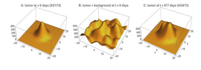
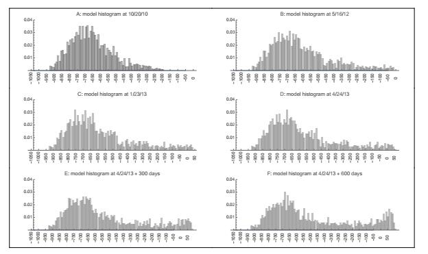
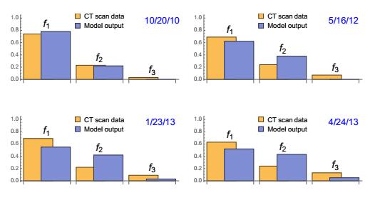
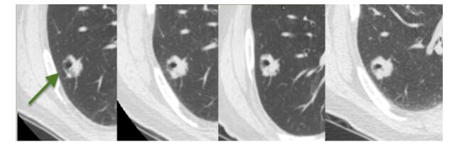
1. | Abdul Alamin, Sankar Prasad Mondal, Kunal Biswas, Shariful Alam, 2020, chapter 6, 9781799837411, 120, 10.4018/978-1-7998-3741-1.ch006 | |
2. | Zhimin Han, Yi Wang, Jinde Cao, Impact of contact heterogeneity on initial growth behavior of an epidemic: Complex network-based approach, 2023, 451, 00963003, 128021, 10.1016/j.amc.2023.128021 |