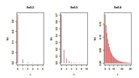
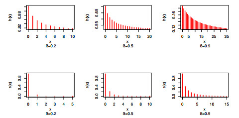
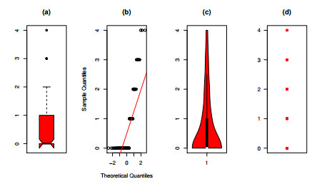
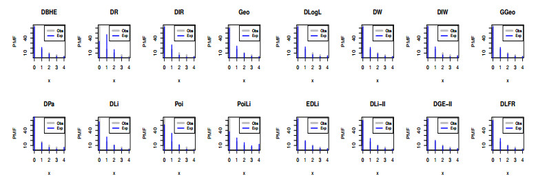
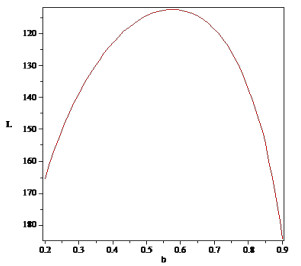
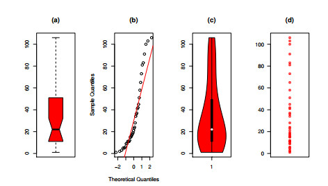
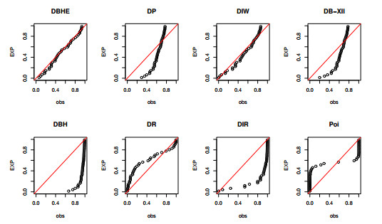
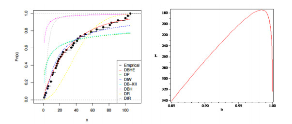
The intertwining relationship between sustainability and discrete probability distributions found its significance in decision-making processes and risk assessment frameworks. Count data modeling and its practical applications have gained attention in numerous research studies. This investigation focused on a particular discrete distribution characterized by a single parameter obtained through the survival discretization method. Statistical attributes of this distribution were accurately explicated using generalized hypergeometric functions. The unveiled characteristics highlighted its suitability for analyzing data displaying "right-skewed" asymmetry and possessing extended "heavy" tails. Its failure rate function effectively addressed scenarios marked by a consistent decrease in rates. Furthermore, it proved to be a valuable tool for probabilistic modeling of over-dispersed data. The study introduced various estimation methods such as maximum product of spacings, Anderson-Darling, right-tail Anderson-Darling, maximum likelihood, least-squares, weighted least-squares, percentile, and Cramer-Von-Mises, offering comprehensive explanations. A ranking simulation study was conducted to evaluate the performance of these estimators, employing ranking techniques to identify the most effective estimator across different sample sizes. Finally, real-world sustainability engineering and medical datasets were analyzed to demonstrate the significance and application of the newly introduced model.
Citation: Khaled M. Alqahtani, Mahmoud El-Morshedy, Hend S. Shahen, Mohamed S. Eliwa. A discrete extension of the Burr-Hatke distribution: Generalized hypergeometric functions, different inference techniques, simulation ranking with modeling and analysis of sustainable count data[J]. AIMS Mathematics, 2024, 9(4): 9394-9418. doi: 10.3934/math.2024458
The intertwining relationship between sustainability and discrete probability distributions found its significance in decision-making processes and risk assessment frameworks. Count data modeling and its practical applications have gained attention in numerous research studies. This investigation focused on a particular discrete distribution characterized by a single parameter obtained through the survival discretization method. Statistical attributes of this distribution were accurately explicated using generalized hypergeometric functions. The unveiled characteristics highlighted its suitability for analyzing data displaying "right-skewed" asymmetry and possessing extended "heavy" tails. Its failure rate function effectively addressed scenarios marked by a consistent decrease in rates. Furthermore, it proved to be a valuable tool for probabilistic modeling of over-dispersed data. The study introduced various estimation methods such as maximum product of spacings, Anderson-Darling, right-tail Anderson-Darling, maximum likelihood, least-squares, weighted least-squares, percentile, and Cramer-Von-Mises, offering comprehensive explanations. A ranking simulation study was conducted to evaluate the performance of these estimators, employing ranking techniques to identify the most effective estimator across different sample sizes. Finally, real-world sustainability engineering and medical datasets were analyzed to demonstrate the significance and application of the newly introduced model.

| [1] |
A. S. Yadav, E. Altun, H. M. Yousof, Burr-Hatke exponential distribution: A decreasing failure rate model, statistical inference and applications, Ann. Data. Sci, 8 (2021), 241–260. https://doi.org/10.1007/s40745-019-00213-8 doi: 10.1007/s40745-019-00213-8

|
| [2] |
M. El-Morshedy, M. S. Eliwa, E. Altun, Discrete Burr-Hatke distribution with properties, estimation methods and regression model, IEEE Access, 8 (2020), 74359–74370. https://doi.org/10.1109/ACCESS.2020.2988431 doi: 10.1109/ACCESS.2020.2988431
|
| [3] |
M. El-Morshedy, A discrete linear-exponential model: Synthesis and analysis with inference to model extreme count data, Axioms, 11 (2022), 531. https://doi.org/10.3390/axioms11100531 doi: 10.3390/axioms11100531
|
| [4] |
H. Krishna, P. S. Pundir, Discrete Burr and discrete Pareto distributions, Statist. Methodol., 6 (2009), 177–188. https://doi.org/10.1016/j.stamet.2008.07.001 doi: 10.1016/j.stamet.2008.07.001
|
| [5] | T. Hussain, M. Ahmad, Discrete inverse Rayleigh distribution, Pakistan J. Statist., 30 (2014), 203. |
| [6] |
M. A. Jazi, C. D. Lai, M. H. Alamatsaz, A discrete inverse Weibull distribution and estimation of its parameters, Statist. Methodol., 7 (2010), 121–132. https://doi.org/10.1016/j.stamet.2009.11.001 doi: 10.1016/j.stamet.2009.11.001
|
| [7] |
E. Gómez-Déniz, E. Calderín-Ojeda, The discrete Lindley distribution: properties and applications, J. Statist. Comput. Simul., 81 (2011), 1405–1416. https://doi.org/10.1080/00949655.2010.487825 doi: 10.1080/00949655.2010.487825
|
| [8] |
J. M. Jia, Z. Z. Yan, X. Y. Peng, A new discrete extended Weibull distribution, IEEE Access, 7 (2019), 175474–175486. https://doi.org/10.1109/ACCESS.2019.2957788 doi: 10.1109/ACCESS.2019.2957788
|
| [9] |
E. Gómez-Déniz, Another generalization of the geometric distribution, Test, 19 (2010), 399–415. https://doi.org/10.1007/s11749-009-0169-3 doi: 10.1007/s11749-009-0169-3
|
| [10] | M. A. Hegazy, R. E. Abd El-Kader, A. A. El-Helbawy, G. R. Al-Dayian, Bayesian estimation and prediction of discrete Gompertz distribution, J. Adv. Math. Comput. Sci., 36 (2021), 1–21. |
| [11] |
V. Nekoukhou, M. H. Alamatsaz, H. Bidram, Discrete generalized exponential distribution of a second type, Statistics, 47 (2013), 876–887. https://doi.org/10.1080/02331888.2011.633707 doi: 10.1080/02331888.2011.633707
|
| [12] |
E. M. Almetwally, S. Dey, S. Nadarajah, An overview of discrete distributions in modelling COVID-19 data sets, Sankhya A, 85 (2023), 1403–1430. https://doi.org/10.1007/s13171-022-00291-6 doi: 10.1007/s13171-022-00291-6
|
| [13] |
A. S. Eldeeb, M. Ahsan-ul-Haq, M. S. Eliwa, A discrete Ramos-Louzada distribution for asymmetric and over-dispersed data with leptokurtic-shaped: Properties and various estimation techniques with inference, AIMS Math., 7 (2022), 1726–1741. https://doi.org/10.3934/math.2022099 doi: 10.3934/math.2022099
|
| [14] |
H. Haj Ahmad, D. A. Ramadan, E. M. Almetwally, Evaluating the discrete generalized Rayleigh distribution: Statistical inferences and applications to real data analysis, Mathematics, 12 (2024), 183. https://doi.org/10.3390/math12020183 doi: 10.3390/math12020183
|
| [15] |
H. M. Aljohani, M. Ahsan-ul-Haq, J. Zafar, E. M. Almetwally, A. S. Alghamdi, E. Hussam, et al., Analysis of COVID-19 data using discrete Marshall-Olkinin length biased exponential: Bayesian and frequentist approach, Sci. Rep., 13 (2023), 12243. https://doi.org/10.1038/s41598-023-39183-6 doi: 10.1038/s41598-023-39183-6
|
| [16] | J. F. Lawless, Statistical Models and Methods for Lifetime Data, Hoboken: John Wiley & Sons, 2011. |
| [17] |
P. Damien, S. Walker, A Bayesian non-parametric comparison of two treatments, Scand. J. Statist., 29 (2002), 51–56. https://doi.org/10.1111/1467-9469.00891 doi: 10.1111/1467-9469.00891
|
Figures(14) / Tables(20)

Khaled M. Alqahtani, Mahmoud El-Morshedy, Hend S. Shahen, Mohamed S. Eliwa. A discrete extension of the Burr-Hatke distribution: Generalized hypergeometric functions, different inference techniques, simulation ranking with modeling and analysis of sustainable count data[J]. AIMS Mathematics, 2024, 9(4): 9394-9418. doi: 10.3934/math.2024458


 DownLoad: