A fast and general algebraic approach to Railway Interlocking System across all train stations

Antonio Hernando; José Luis Galán-García; Gabriel Aguilera-Venegas; Antonio Hernando; José Luis Galán-García; Gabriel Aguilera-Venegas

doi:10.3934/math.2024373

AIMS Mathematics

2024, Volume 9, Issue 3: 7673-7710. doi: 10.3934/math.2024373

Previous Article Next Article

Research article Special Issues

A fast and general algebraic approach to Railway Interlocking System across all train stations

1.
Depto. de Sistemas Informáticos, E.T.S.I. de Sistemas Informáticos, Universidad Politécnica de Madrid, Madrid, Spain
2.
Departamento de Matemática Aplicada, Escuela de Ingenierías Industriales, Universidad de Málaga, Málaga, Spain

Received: 12 October 2023 Revised: 06 February 2024 Accepted: 19 February 2024 Published: 22 February 2024
MSC : 13P05

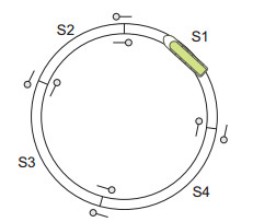
Railway interlocking systems are crucial safety components in rail transportation, designed to prevent train collisions by regulating switch positions and signal indications. These systems delineate potential train movements within a railway station by connecting sections into routes, which are further divided into blocks. To ensure safety, the system prohibits the simultaneous allocation of the same block or intersecting routes to multiple trains. In this study, we characterize the 'interlocking problem' as a safety verification task for a single real-time station configuration, rather than a 'command and control' function. This is a matter of verification, not solution, typically managed by an interlocking system that receives movement authority requests. Over the years, we have developed various algebraic models to address this issue, suggesting the potential use of computer algebra systems in implementing interlocking systems. However, some of these models exhibit limitations. In this paper, we propose a novel algebraic model for decision-making in railway interlocking systems that overcomes the limitations of previous approaches, making it suitable for large railway stations. Our primary objective is to offer a mathematical solution to interlocking problems in linear time, which our approach accomplishes.
- railway interlocking system,
- computer algebra,
- decision making,
- commutative algebra
Citation: Antonio Hernando, José Luis Galán-García, Gabriel Aguilera-Venegas. A fast and general algebraic approach to Railway Interlocking System across all train stations[J]. AIMS Mathematics, 2024, 9(3): 7673-7710. doi: 10.3934/math.2024373

Related Papers:

Abstract

Railway interlocking systems are crucial safety components in rail transportation, designed to prevent train collisions by regulating switch positions and signal indications. These systems delineate potential train movements within a railway station by connecting sections into routes, which are further divided into blocks. To ensure safety, the system prohibits the simultaneous allocation of the same block or intersecting routes to multiple trains. In this study, we characterize the 'interlocking problem' as a safety verification task for a single real-time station configuration, rather than a 'command and control' function. This is a matter of verification, not solution, typically managed by an interlocking system that receives movement authority requests. Over the years, we have developed various algebraic models to address this issue, suggesting the potential use of computer algebra systems in implementing interlocking systems. However, some of these models exhibit limitations. In this paper, we propose a novel algebraic model for decision-making in railway interlocking systems that overcomes the limitations of previous approaches, making it suitable for large railway stations. Our primary objective is to offer a mathematical solution to interlocking problems in linear time, which our approach accomplishes.

References

[1]	N. Bešinović, Resilience in railway transport systems: a literature review and research agenda, Transport Rev., 40 (2020), 457–478. https://doi.org/10.1080/01441647.2020.1728419 doi: 10.1080/01441647.2020.1728419
[2]	Y. Zhou, J. Wang, H. Yang, Resilience of transportation systems: concepts and comprehensive review, IEEE Trans. Intell. Transp. Syst., 20 (2019), 4262–4276. https://doi.org/10.1109/TITS.2018.2883766 doi: 10.1109/TITS.2018.2883766
[3]	H. Lian, X. Wang, A. Sharma, M. A. Shah, Application and study of artificial intelligence in railway signal interlocking fault, Informatica, 46 (2022), 343–354. https://doi.org/10.31449/inf.v46i3.3961 doi: 10.31449/inf.v46i3.3961
[4]	A. Fantechi, G. Gori, A. E. Haxthausen, C. Limbrée, Compositional verification of railway interlockings: comparison of two methods, in Reliability, Safety, and Security of Railway Systems. Modelling, Analysis, Verification, and Certification, (2022), 3–19. https://doi.org/10.1007/978-3-031-05814-1_1
[5]	G. Lukács, T. Bartha, Conception of a formal model-based methodology to support railway engineers in the specification and verification of interlocking systems, in 2022 IEEE 16th International Symposium on Applied Computational Intelligence and Informatics (SACI), (2022), 000283–000288. https://doi.org/10.1109/SACI55618.2022.9919532
[6]	K. Winter, W. Johnston, P. Robinson, P. Strooper, L. van den Berg, Tool support for checking railway interlocking designs, in 10th Australian Workshop on Safety Re-lated Programmable Systems (SCS'05), Australian Computer Society, Sydney, 55 (2006), 101–107. Available from: https://crpit.scem.westernsydney.edu.au/confpapers/CRPITV55Winter.pdf.
[7]	J. Peleska, N. Krafczyk, A. E. Haxthausen, R. Pinger, Efficient data validation for geographical interlocking systems, Formal Aspects Comput., 33 (2021), 925–955. https://doi.org/10.1007/s00165-021-00551-6 doi: 10.1007/s00165-021-00551-6
[8]	A. Fantechi, A. E. Haxthausen, M. B. R. Nielsen, Model checking geographically distributed interlocking systems using UMC, in 2017 25th Euromicro International Conference on Parallel, Distributed and Network-based Processing (PDP), (2017), 278–286. https://doi.org/10.1109/PDP.2017.66
[9]	E. Roanes-Lozano, L. M. Laita, An applicable topology-independent model for railway interlocking systems, Math. Comput. Simul., 45 (1998), 175–183. https://doi.org/10.1016/S0378-4754(97)00093-1 doi: 10.1016/S0378-4754(97)00093-1
[10]	E. Roanes-Lozano, E. Roanes-Macías, L. Laita, Railway interlocking systems and Gröbner bases, Math. Comput. Simul., 51 (2000), 473–481. https://doi.org/10.1016/S0378-4754(99)00137-8 doi: 10.1016/S0378-4754(99)00137-8
[11]	E. Roanes-Lozano, A. Hernando, J. A. Alonso, L. M. Laita, A logic approach to decision taking in a railway interlocking system using Maple, Math. Comput. Simul., 82 (2011), 15–28. https://doi.org/10.1016/j.matcom.2010.05.024 doi: 10.1016/j.matcom.2010.05.024
[12]	A. Hernando, E. Roanes-Lozano, R. Maestre-Martínez, J. Tejedor, A logic-algebraic approach to decision taking in a railway interlocking system, Ann. Math. Artif. Intell., 65 (2012), 317–328. https://doi.org/10.1007/s10472-012-9321-y doi: 10.1007/s10472-012-9321-y
[13]	E. Roanes-Lozano, J. A. Alonso, A. Hernando, An approach from answer set programming to decision making in a railway interlocking system, Rev. R. Acad. Cienc. Exactas, Fis. Nat. Ser. A Mat., 108 (2014), 973–987. https://doi.org/10.1007/s13398-013-0155-1 doi: 10.1007/s13398-013-0155-1
[14]	A. Hernando, R. Maestre, E. Roanes-Lozano, A new algebraic approach to decision making in a railway interlocking system based on preprocess, Math. Probl. Eng., 2018 (2018), 4982974. https://doi.org/10.1155/2018/4982974 doi: 10.1155/2018/4982974
[15]	A. Hernando, E. Roanes-Lozano, An algebraic model for implementing expert systems based on the knowledge of different experts, Math. Comput. Simul., 107 (2015), 92–107. https://doi.org/10.1016/j.matcom.2014.05.003 doi: 10.1016/j.matcom.2014.05.003
[16]	A. Hernando, A., E. Roanes-Lozano, J.L. Galán-García, G. Aguilera-Venegas, Decision making in railway interlocking systems based on calculating the remainder of dividing a polynomial by a set of polynomials, Electron. Res. Arch., 31 (2023), 6160–6196. https://10.3934/era.2023313
[17]	D. Cox, J. Little, D. O'Shea, Ideals, Varieties and Algorithms, Springer, 2015. Available from: https://link.springer.com/book/10.1007/978-3-319-16721-3.
[18]	J. Abbott, A. M. Bigatti, CoCoALib: a C++ library for doing Computations in Commutative Algebra, 2019. Available from: http://cocoa.dima.unige.it/cocoalib.
[19]	D. Bjørner, The FMERail/TRain Annotated Rail Bibliography, 1999. Available from: http://www2.imm.dtu.dk/db/fmerail/fmerail/.
[20]	M. J. Morley, Modelling British Rail's Interlocking Logic: Geographic Data Correctness, LFCS, Department of Computer Science, University of Edinburgh, 1991.
[21]	K. Nakamatsu, Y. Kiuchi, A. Suzuki, EVALPSN based railway interlocking simulator, in Knowledge-Based Intelligent Information and Engineering Systems, Berlin - Heidelberg, (2004), 961–967. https://doi.org/10.1007/978-3-540-30133-2_127
[22]	A. Janota, Using Z specification for railway interlocking safety, Period. Polytech. Transp. Eng., 28 (2000), 39–53. Available from: https://pp.bme.hu/tr/article/view/1963.
[23]	K. M. Hansen, Formalising railway interlocking systems, in Nordic Seminar on Dependable Computing Systems, Lyngby, (1994), 83–94.
[24]	M. Montigel, Modellierung und Gewährleistung von Abhängigkeiten in Eisenbahnsicherungsanlagen, Ph.D. Thesis, ETH Zurich, Zurich, 1994. Available from: http://www.inf.ethz.ch/research/disstechreps/theses.
[25]	X. Chen, H. Huang, Y. He, Automatic generation of relay logic for interlocking system based on statecharts, in 2010 Second World Congress on Software Engineering, (2010), 183–188. https://doi.org/10.1109/WCSE.2010.31
[26]	X. Chen, Y. He, H. Huang, An approach to automatic development of interlocking logic based on Statechart, Enterp. Inf. Syst., 5 (2011), 273–286. https://doi.org/10.1080/17517575.2011.575475 doi: 10.1080/17517575.2011.575475
[27]	X. Chen, Y. He, H. Huang, A component-based topology model for railway interlocking systems, Math. Comput. Simul., 81 (2011), 1892–1900. https://doi.org/10.1016/j.matcom.2011.02.007 doi: 10.1016/j.matcom.2011.02.007
[28]	B. Luteberget, C. Johansen, Efficient verification of railway infrastructure designs against standard regulations, Formal Methods Syst. Des., 52 (2018), 1–32. https://doi.org/10.1007/s10703-017-0281-z doi: 10.1007/s10703-017-0281-z
[29]	M. Bosschaart, E. Quaglietta, B. Janssen, R. M. P. Goverde, Efficient formalization of railway interlocking data in RailML, Inf. Syst., 49 (2015), 126–141. https://doi.org/10.1016/j.is.2014.11.007 doi: 10.1016/j.is.2014.11.007
[30]	E. Roanes-Lozano, L. M. Laita, E. Roanes-Macías, An application of an AI methodology to railway interlocking systems using computer algebra, in Tasks and Methods in Applied Artificial Intelligence, (1998), 687–696. https://doi.org/10.1007/3-540-64574-8_455
[31]	B. Buchberger, An algorithm for finding the basis elements of the residue class ring of a zero dimensional polynomial ideal, J. Symb. Comput., 41 (2006), 475–511. https://doi.org/10.1016/j.jsc.2005.09.007 doi: 10.1016/j.jsc.2005.09.007
[32]	M. Davis, G. Logemann, D. Loveland, A machine program for theorem-proving, Commun. ACM, 5 (1962), 394–397. https://doi.org/10.1145/368273.368557 doi: 10.1145/368273.368557
[33]	Ministerio de Transportes, Movilidad y Agenda Urbana, Estudio Informativo del Nuevo Complejo Ferroviario de la Estación de Madrid-Chamartín. Available from: https://www.mitma.gob.es/ferrocarriles/estudios-en-tramite/estudios-y-proyectos-entramite/chamartin.
[34]	Anonyous, Adjudicada la Modificación de Las Instalaciones de Seguridad, ERTMS, Comunicaciones y Energía de Madrid-Chamartín, Vía Libre, 2021. Available from: https://www.vialibre-ffe.com/noticias.asp?not = 33047 & cs = infr.
[35]	G. Aguilera-Venegas, J. L. Galán-García, E. Mérida-Casermeiro, P. Rodríguez-Cielos, An accelerated-time simulation of baggage traffic in an airport terminal, Math. Comput. Simul., 104 (2014), 58–66. https://doi.org/10.1016/j.matcom.2013.12.009 doi: 10.1016/j.matcom.2013.12.009
[36]	G. Aguilera, J. L. Galán, J. M. García, E. Mérida, P. Rodríguez, An accelerated-time simulation of car traffic on a motorway using a CAS, Math. Comput. Simul., 104 (2014), 21–30. https://doi.org/10.1016/j.matcom.2012.03.010 doi: 10.1016/j.matcom.2012.03.010
[37]	J. L. Galán-García, G. Aguilera-Venegas, M. Á. Galán-García, P. Rodríguez-Cielos, A new Probabilistic Extension of Dijkstra's Algorithm to simulate more realistic traffic flow in a smart city, Appl. Math. Comput., 267 (2015), 780–789. https://doi.org/10.1016/j.amc.2014.11.076 doi: 10.1016/j.amc.2014.11.076
[38]	J. L. Galán-García, G. Aguilera-Venegas, P. Rodríguez-Cielos, An accelerated-time simulation for traffic flow in a smart city, J. Comput. Appl. Math., 270 (2014), 557–563. https://doi.org/10.1016/j.cam.2013.11.020 doi: 10.1016/j.cam.2013.11.020
[39]	A. Iliasov, D. Taylor, L. Laibinis, A. B. Romanovsky, SafeCap: from formal verification of railway interlocking to its certification, 2021.
[40]	J. Pachl, Railway signalling principles, 2021. Available from: http://www.joernpachl.de/rsp.htm.
[41]	A. Borälv, Case study: formal verification of a computerized railway interlocking, Formal Aspects Comput., 10 (1998), 338–360. https://doi.org/10.1007/s001650050021 doi: 10.1007/s001650050021
[42]	Anonymous, Proyecto y obra del enclavamiento electrónico de la estación de Madrid-Atocha, Proyecto Técnico, Siemens, Madrid, 1988.
[43]	Anonymous, Microcomputer interlocking hilversum, Siemens, Munich, 1986.
[44]	Anonymous, Microcomputer interlocking rotterdam, Siemens, Munich, 1989.
[45]	Anonymous, Puesto de enclavamiento con microcomputadoras de la estación de Chiasso de los SBB, Siemens, Munich, 1989.
[46]	L. Villamandos, Sistema informático concebido por Renfe para diseñar los enclavamientos, Vía Libre, 348 (1993), 65.

Reader Comments

Your name:*

Email:*
© 2024 the Author(s), licensee AIMS Press. This is an open access article distributed under the terms of the Creative Commons Attribution License (http://creativecommons.org/licenses/by/4.0)